Concept
Contents
Concept#
Notations#
Definition 118 (Underlying Distributions)
\(\mathcal{X}\): Input space consists of all possible inputs \(\mathbf{x} \in \mathcal{X}\).
\(\mathcal{Y}\): Label space = \(\{1, 2, \ldots, K\}\) where \(K\) is the number of classes.
The mapping between \(\mathcal{X}\) and \(\mathcal{Y}\) is given by \(c: \mathcal{X} \rightarrow \mathcal{Y}\) where \(c\) is called concept according to the PAC learning theory.
\(\mathcal{D}\): The fixed but unknown distribution of the data. Usually, this refers to the joint distribution of the input and the label,
\[\begin{split} \mathcal{D} &= \mathbb{P}(\mathcal{X}, \mathcal{Y} ; \boldsymbol{\theta}) \\ &= \mathbb{P}_{\{\mathcal{X}, \mathcal{Y} ; \boldsymbol{\theta}\}}(\mathbf{x}, y) \end{split}\]where \(\mathbf{x} \in \mathcal{X}\) and \(y \in \mathcal{Y}\), and \(\boldsymbol{\theta}\) is the parameter vector of the distribution \(\mathcal{D}\).
Definition 119 (Dataset)
Now, consider a dataset \(\mathcal{D}_{\{\mathbf{x}, y\}}\) consisting of \(N\) samples (observations) and \(D\) predictors (features) drawn jointly and indepedently and identically distributed (i.i.d.) from \(\mathcal{D}\). Note we will refer to the dataset \(\mathcal{D}_{\{\mathbf{x}, y\}}\) with the same notation as the underlying distribution \(\mathcal{D}\) from now on.
The training dataset \(\mathcal{D}\) can also be represented compactly as a set:
\[\begin{split} \begin{align*} \mathcal{D} \overset{\mathbf{def}}{=} \mathcal{D}_{\{\mathbf{x}, y\}} &= \left\{\mathbf{x}^{(n)}, y^{(n)}\right\}_{n=1}^N \\ &= \left\{\left(\mathbf{x}^{(1)}, y^{(1)}\right), \left(\mathbf{x}^{(2)}, y^{(2)}\right), \cdots, \left(\mathbf{x}^{(N)}, y^{(N)}\right)\right\} \\ &= \left\{\mathbf{X}, \mathbf{y}\right\} \end{align*} \end{split}\]where we often subscript \(\mathbf{x}\) and \(y\) with \(n\) to denote the \(n\)-th sample from the dataset, i.e. \(\mathbf{x}^{(n)}\) and \(y^{(n)}\). Most of the times, \(\mathbf{x}^{(n)}\) is bolded since it represents a vector of \(D\) number of features, while \(y^{(n)}\) is not bolded since it is a scalar, though it is not uncommon for \(y^{(n)}\) to be bolded as well if you represent it with K-dim one-hot vector.
For the n-th sample \(\mathbf{x}^{(n)}\), we often denote the \(d\)-th feature as \(x_d^{(n)}\) and the representation of \(\mathbf{x}^{(n)}\) as a vector as:
\[ \mathbf{x}^{(n)} \in \mathbb{R}^{D} = \begin{bmatrix} x_1^{(n)} & x_2^{(n)} & \cdots & x_D^{(n)} \end{bmatrix}_{D \times 1} \]is a sample of size \(D\), drawn (jointly with \(y\)) \(\textbf{i.i.d.}\) from \(\mathcal{D}\).
We often add an extra feature \(x_0^{(n)} = 1\) to \(\mathbf{x}^{(n)}\) to represent the bias term. i.e.
\[ \mathbf{x}^{(n)} \in \mathbb{R}^{D+1} = \begin{bmatrix} x_0^{(n)} & x_1^{(n)} & x_2^{(n)} & \cdots & x_D^{(n)} \end{bmatrix}_{(D+1) \times 1} \]For the n-th sample’s label \(y^{(n)} \overset{\mathbf{def}}{=} c(\mathbf{x}^{(n)})\), if we were to represent it as K-dim one-hot vector, we would have:
\[ y^{(n)} \in \mathbb{R}^{K} = \begin{bmatrix} 0 & 0 & \cdots & 1 & \cdots & 0 \end{bmatrix}_{K \times 1} \]where the \(1\) is at the \(k\)-th position, and \(k\) is the class label of the n-th sample.
Everything defined above is for one single sample/data point, to represent it as a matrix, we can define a design matrix \(\mathbf{X}\) and a label vector \(\mathbf{y}\) as follows,
\[\begin{split} \begin{aligned} \mathbf{X} \in \mathbb{R}^{N \times D} &= \begin{bmatrix} \mathbf{x}^{(1)} \\ \mathbf{x}^{(2)} \\ \vdots \\ \mathbf{x}^{(N)} \end{bmatrix} = \begin{bmatrix} x_1^{(1)} & x_2^{(1)} & \cdots & x_D^{(1)} \\ x_1^{(2)} & x_2^{(2)} & \cdots & x_D^{(2)} \\ \vdots & \vdots & \ddots & \vdots \\ x_1^{(N)} & x_2^{(N)} & \cdots & x_D^{(N)} \end{bmatrix}_{N \times D} \\ \end{aligned} \end{split}\]as the matrix of all samples. Note that each row is a sample and each column is a feature. We can append a column of 1’s to the first column of \(\mathbf{X}\) to represent the bias term.
In this section, we also talk about random vectors \(\mathbf{X}\) so we will replace the design matrix \(\mathbf{X}\) with \(\mathbf{A}\) to avoid confusion.
Subsequently, for the label vector \(\mathbf{y}\), we can define it as follows,
\[\begin{split} \begin{aligned} \mathbf{y} \in \mathbb{R}^{N} = \begin{bmatrix} y^{(1)} \\ y^{(2)} \\ \vdots \\ y^{(N)} \end{bmatrix} \end{aligned} \end{split}\]
Example 25 (Joint Distribution Example)
For example, if the number of features, \(D = 2\), then let’s say
consists of two Gaussian random variables, with \(\mu_1\) and \(\mu_2\) being the mean of the two distributions, and \(\sigma_1\) and \(\sigma_2\) being the variance of the two distributions; furthermore, \(Y^{(n)}\) is a Bernoulli random variable with parameter \(\boldsymbol{\pi}\), then we have
where \(\boldsymbol{\mu} = \begin{bmatrix} \mu_1 & \mu_2 \end{bmatrix}\) and \(\boldsymbol{\sigma} = \begin{bmatrix} \sigma_1 & \sigma_2 \end{bmatrix}\).
Remark 35 (Some remarks)
From now on, we will refer the realization of \(Y\) as \(k\) instead.
For some sections, when I mention \(\mathbf{X}\), it means the random vector which resides in the \(D\)-dimensional space, not the design matrix. This also means that this random vector refers to a single sample, not the entire dataset.
Definition 120 (Joint and Conditional Probability)
We are often interested in finding the probability of a label given a sample,
where
is a random vector and its realizations,
and therefore, \(\mathbf{X}\) can be characterized by an \(D\)-dimensional PDF
and
is a discrete random variable (in our case classification) and its realization respectively, and therefore, \(Y\) can be characterized by a discrete PDF (PMF)
Note that we are talking about one single sample tuple \(\left(\mathbf{x}, y\right)\) here. I did not index the sample tuple with \(n\) because this sample can be any sample in the unknown distribution \(\mathbb{P}_{\mathcal{X}, \mathcal{Y}}(\mathbf{x}, y)\) and not only from our given dataset \(\mathcal{D}\).
Definition 121 (Likelihood)
We denote the likelihood function as \(\mathbb{P}(\mathbf{X} = \mathbf{x} \mid Y = k)\), which is the probability of observing \(\mathbf{x}\) given that the sample belongs to class \(Y = k\).
Definition 122 (Prior)
We denote the prior probability of class \(k\) as \(\mathbb{P}(Y = k)\), which usually follows a discrete distribution such as the Categorical distribution.
Definition 123 (Posterior)
We denote the posterior probability of class \(k\) given \(\mathbf{x}\) as \(\mathbb{P}(Y = k \mid \mathbf{X} = \mathbf{x})\).
Definition 124 (Marginal Distribution and Normalization Constant)
We denote the normalizing constant as \(\mathbb{P}(\mathbf{X} = \mathbf{x}) = \sum_{k=1}^K \mathbb{P}(Y = k) \mathbb{P}(\mathbf{X} = \mathbf{x} \mid Y = k)\).
Discriminative vs Generative#
Discriminative classifiers model the conditional distribution \(\mathbb{P}(Y = k \mid \mathbf{X} = \mathbf{x})\). This means we are modelling the conditional distribution of the target \(Y\) given the input \(\mathbf{x}\).
Generative classifiers model the conditional distribution \(\mathbb{P}(\mathbf{X} = \mathbf{x} \mid Y = k)\). This means we are modelling the conditional distribution of the input \(\mathbf{X}\) given the target \(Y\). Then we can use Bayes’ rule to compute the conditional distribution of the target \(Y\) given the input \(\mathbf{X}\).
Both the target \(Y\) and the input \(\mathbf{X}\) are random variables in the generative model. In the discriminative model, only the target \(Y\) is a random variable as the input \(\mathbf{X}\) is fixed (we do not need to estimate anything about the input \(\mathbf{X}\)).
For example, Logistic Regression models the target \(Y\) as a function of predictor’s \(\mathbf{X} = \begin{bmatrix}X_1 \\ X_2 \\ \vdots \\X_D \end{bmatrix}\).
Naive bayes models both the target \(Y\) and the predictors \(\mathbf{X}\) as a function of each other. This means we are modelling the joint distribution of the target \(Y\) and the predictors \(\mathbf{X}\).
Naive Bayes Setup#
Let
be the dataset with \(N\) samples and \(D\) predictors.
All samples are assumed to be independent and identically distributed (i.i.d.) from the unknown but fixed joint distribution \(\mathbb{P}(\mathcal{X}, \mathcal{Y} ; \boldsymbol{\theta})\),
where \(\boldsymbol{\theta}\) is the parameter vector of the joint distribution. See Example 25 for an example of such.
Inference/Prediction#
Before we look at the fitting/estimating process, let’s look at the inference/prediction process.
Suppose the problem at hand has \(K\) classes, \(k = 1, 2, \cdots, K\), where \(k\) is the index of the class.
Then, to find the class of a new test sample \(\mathbf{x}^{(q)} \in \mathbb{R}^{D}\) with \(D\) features, we can compute the conditional probability of each class \(Y = k\) given the sample \(\mathbf{x}^{(q)}\):
Algorithm 1 (Naive Bayes Inference Algorithm)
Compute the conditional probability of each class \(Y = k\) given the sample \(\mathbf{x}^{(q)}\):
(73)#\[ \mathbb{P}(Y = k \mid \mathbf{X} = \mathbf{x}^{(q)}) = \dfrac{\mathbb{P}(Y = k) \mathbb{P}(\mathbf{X} = \mathbf{x}^{(q)} \mid Y = k)}{\mathbb{P}(\mathbf{X} = \mathbf{x}^{(q)})} \quad \text{for } k = 1, 2, \cdots, K \]Choose the class \(k\) that maximizes the conditional probability:
(74)#\[ \hat{y}^{(q)} = \arg\max_{k=1}^K \mathbb{P}(Y = k \mid \mathbf{X} = \mathbf{x}^{(q)}) \]The observant reader would have noticed that the normalizing constant \(\mathbb{P}\left(X = \mathbf{x}^{(q)}\right)\) is the same for all \(k\). Therefore, we can ignore it and simply choose the class \(k\) that maximizes the numerator of the conditional probability in (73):
(75)#\[ \hat{y}^{(q)} = \arg\max_{k=1}^K \mathbb{P}(Y = k) \mathbb{P}(\mathbf{X} = \mathbf{x}^{(q)} \mid Y = k) \]since where the normalizing constant is ignored, the conditional probability
(76)#\[ \mathbb{P}(Y = k \mid \mathbf{X} = \mathbf{x}^{(q)}) \propto \mathbb{P}(Y = k) \mathbb{P}(\mathbf{X} = \mathbf{x}^{(q)} \mid Y = k) \]by a constant factor \(\mathbb{P}(\mathbf{X} = \mathbf{x}^{(q)})\).
Note however, to recover the normalizing constant is easy, since the numerator \(\mathbb{P}(Y = k) \mathbb{P}(\mathbf{X} = \mathbf{x}^{(q)} \mid Y = k) \) must sum up to 1 over all \(k\), and therefore, the normalizing constant is simply \(\mathbb{P}(\mathbf{X} = \mathbf{x}^{(q)}) = \sum_{k=1}^K \mathbb{P}(Y = k) \mathbb{P}(\mathbf{X} = \mathbf{x}^{(q)} \mid Y = k)\).
Expressing it in vector form, we have
(77)#\[\begin{split} \begin{aligned} \hat{\mathbf{y}} &= \arg\max_{k=1}^K \begin{bmatrix} \mathbb{P}(Y=1) \mathbb{P}(\mathbf{X} = \mathbf{x}\mid Y = 1) \\ \mathbb{P}(Y=2) \mathbb{P}(\mathbf{X} = \mathbf{x}\mid Y = 2) \\ \vdots \\ \mathbb{P}(Y=K) \mathbb{P}(\mathbf{X} = \mathbf{x} \mid Y = K) \end{bmatrix}_{K \times 1} \\ &= \arg\max_{k=1}^K \begin{bmatrix} \mathbb{P}(Y=1) \\ \mathbb{P}(Y=2) \\ \cdots \\ \mathbb{P}(Y=K) \end{bmatrix}\circ \begin{bmatrix} \mathbb{P}(\mathbf{X} = \mathbf{x} \mid Y = 1) \\ \mathbb{P}(\mathbf{X} = \mathbf{x}\mid Y = 2) \\ \vdots \\ \mathbb{P}(\mathbf{X} = \mathbf{x} \mid Y = K) \end{bmatrix} \\ &= \arg\max_{k=1}^K \mathbf{M_1} \circ \mathbf{M_2} \\ &= \arg\max_{k=1}^K \mathbf{M_1} \circ \mathbf{M_3} \\ \end{aligned} \end{split}\]where
(78)#\[\begin{split} \mathbf{M_1} = \begin{bmatrix} \mathbb{P}(Y = 1) \\ \mathbb{P}(Y = 2) \\ \vdots \\ \mathbb{P}(Y = K) \end{bmatrix}_{K \times 1} \end{split}\](79)#\[\begin{split} \mathbf{M_2} = \begin{bmatrix} \mathbb{P}(\mathbf{X} = \mathbf{x} \mid Y = 1) \\ \mathbb{P}(\mathbf{X} = \mathbf{x} \mid Y = 2) \\ \vdots \\ \mathbb{P}(\mathbf{X} = \mathbf{x} \mid Y = K) \end{bmatrix}_{K \times 1} \end{split}\]and
(80)#\[\begin{split} \mathbf{M_3} &= \begin{bmatrix} \mathbb{P}(X_1 = x_1 \mid Y = 1 ; \theta_{11}) & \mathbb{P}(X_2 = x_2 \mid Y = 1 ; \theta_{12}) & \cdots & \mathbb{P}(X_D = x_D \mid Y = 1 ; \theta_{1D}) \\ \mathbb{P}(X_1 = x_1 \mid Y = 2 ; \theta_{21}) & \mathbb{P}(X_2 = x_2 \mid Y = 2 ; \theta_{22}) & \cdots & \mathbb{P}(X_D = x_D \mid Y = 2 ; \theta_{2D}) \\ \vdots & \vdots & \ddots & \vdots \\ \mathbb{P}(X_1 = x_1 \mid Y = K ; \theta_{K1}) & \mathbb{P}(X_2 = x_2 \mid Y = K ; \theta_{K2}) & \cdots & \mathbb{P}(X_D = x_D \mid Y = K ; \theta_{KD}) \end{bmatrix}_{K \times D} \\ \end{split}\]Note superscript \(q\) is removed for simplicity, and \(\circ\) is the element-wise (Hadamard) product. We will also explain why we replace \(\mathbf{M_2}\) with \(\mathbf{M_3}\) in Conditional Independence.
Now if we just proceed to estimate the conditional probability \(\mathbb{P}(Y = k \mid \mathbf{X} = \mathbf{x}^{(q)})\), we will need to estimate the joint probability \(\mathbb{P}(X = \mathbf{x}^{(q)}, Y = k)\), since by definition, we have
which is intractable1.
However, if we can estimate the conditional probability (likelihood) \(\mathbb{P}(\mathbf{X} = \mathbf{x}^{(q)} \mid Y = k)\) and the prior probability \(\mathbb{P}(Y = k)\), then we can use Bayes’ rule to compute the posterior conditional probability \(\mathbb{P}(Y = k \mid \mathbf{X} = \mathbf{x}^{(q)})\).
The Naive Bayes Form#
Quoted from Wikipedia, it is worth noting that there’s a few forms of Naive Bayes:
Simple Form#
If \(X\) is continuous and \(Y\) is discrete,
where each \(f\) is a density function.
If \(X\) is discrete and \(Y\) is continuous,
If both \(X\) and \(Y\) are continuous,
Extended form#
A continuous event space is often conceptualized in terms of the numerator terms. It is then useful to eliminate the denominator using the law of total probability. For \(f_Y(y)\), this becomes an integral:
The Naive Bayes Assumptions#
In this section, we talk about some implicit and explicit assumptions of the Naive Bayes model.
Independent and Identically Distributed (i.i.d.)#
In supervised learning, implicitly or explicitly, one always assumes that the training set
is composed of \(N\) input/response tuples
that are independently drawn from the same (identical) joint distribution
with
where \(\mathbb{P}(Y = y \mid \mathbf{X} = \mathbf{x})\) is the conditional probability of \(Y\) given \(\mathbf{X}\), the relationship that the learner algorithm/concept \(c\) is trying to capture.
Definition 125 (The i.i.d. Assumption)
Mathematically, this i.i.d. assumption writes (also defined in Definition 31):
and we sometimes denote
The confusion in the i.i.d. assumption is that we are not talking about the individual random variables \(X_1^{(n)}, X_2^{(n)}, \ldots, X_D^{(n)}\) here, but the entire random vector \(\mathbf{X}^{(n)}\).
This means there is no assumption of \(X_1^{(n)}, X_2^{(n)}, \ldots, X_D^{(n)}\) being i.i.d.. Instead, the samples \(\mathbf{X}^{(1)}, \mathbf{X}^{(2)}, \ldots, \mathbf{X}^{(N)}\) are i.i.d..
Conditional Independence#
The core assumption of the Naive Bayes model is that the predictors \(\mathbf{X}\) are conditionally independent given the class label \(Y\).
But how did we arrive at the conditional independence assumption? Let’s look at what we wanted to achieve in the first place.
Recall that our goal in Inference/Prediction is to find the class \(k \in \{1, 2, \cdots, K\}\) that maximizes the posterior probability \(\mathbb{P}(Y = k \mid \mathbf{X} = \mathbf{x}^{(q)} ; \boldsymbol{\theta})\).
We have seen earlier in Algorithm 1 that since the denominator is constant for all \(k\), we can ignore it and just maximize the numerator.
This suggests we need to find estimates for both the prior and the likelihood. This of course involves us finding the \(\boldsymbol{\pi}\) and \(\boldsymbol{\theta}_{\{\mathbf{X} \mid Y\}}\) that maximize the likelihood function2, which we will talk about later.
In order to meaningfully optimize the expression, we need to decompose the expression (83) into its components that contain the parameters we want to estimate.
which is actually the joint distribution of \(\mathbf{X}\) and \(Y\)3.
This joint distribution expression (84) can be further decomposed by the chain rule of probability4 as
This alone does not get us any further, we still need to estimate roughly \(2^{D}\) parameters5, which is computationally expensive. Not to forget that we need to estimate for each class \(k \in \{1, 2, 3, \ldots, K\}\) which has a complexity of \(\sim \mathcal{O}(2^DK)\).
Remark 36 (Why \(2^D\) parameters?)
Let’s simplify the problem by assuming each feature \(X_d\) and the class label \(Y\) are binary random variables, i.e. \(X_d \in \{0, 1\}\) and \(Y \in \{0, 1\}\).
Then \(\mathbb{P}(Y, X_1, X_2, \ldots X_D)\) is a joint distribution of \(D+1\) random variables, each with \(2\) values.
This means the sample space of \(\mathbb{P}(Y, X_1, X_2, \ldots X_D)\) is
which has \(2^{D+1}\) elements. To really get the exact joint distribution, we need to estimate the probability of each element in the sample space, which is \(2^{D+1}\) parameters.
This has two caveats:
There are too many parameters to estimate, which is computationally expensive. Imagine if \(D\) is 1000, we need to estimate \(2^{1000}\) parameters, which is infeasible.
Even if we can estimate all the parameters, we are essentially overfitting the data by memorizing the training data. There is no learning involved.
This is where the “Naive” assumption comes in. The Naive Bayes’ classifier assumes that the features are conditionally independent6 given the class label.
More formally stated,
Definition 126 (Conditional Independence)
with this assumption, we can further simplify expression (85) as
More precisely, after the simplification in (87), the argmax expression in (73) can be written as
Consequently, our argmax expression in (75) can be written as
We also make some updates to the vector form (77) by updating \(\mathbf{M_2}\) to:
To easily recover each row of \(\mathbf{M_2}\), it is efficient to define a \(K \times D\) matrix, denoted \(\mathbf{M_3}\)
where we can easily recover each row of \(\mathbf{M_2}\) by taking the product of the corresponding row of \(\mathbf{M_3}\).
Parameter Vector#
In the last section on Conditional Independence, we indicated parameters in the expressions. Here we discuss a little on this newly introduced notation.
Each \(\pi_k\) of \(\boldsymbol{\pi}\) refers to the prior probability of class \(k\), and \(\theta_{kd}\) refers to the parameter of the class conditional density for class \(k\) and feature \(d\)7. Furthermore, the boldsymbol \(\boldsymbol{\theta}\) is the parameter vector,
Definition 127 (The Parameter Vector)
There is not much to say about the categorical component \(\boldsymbol{\pi}\), since we are just estimating the prior probabilities of the classes.
The parameter vector (matrix) \(\boldsymbol{\theta}_{\{\mathbf{X} \mid Y\}}=\{\theta_{kd}\}_{k=1, d=1}^{K, D}\) is a bit more complicated. It resides in the \(\mathbb{R}^{K \times D}\) space, where each element \(\theta_{kd}\) is the parameter associated with feature \(d\) conditioned on class \(k\).
So if \(K=3\) and \(D=2\), then the parameter vector \(\boldsymbol{\theta}\) is a \(3 \times 2\) matrix, i.e.
This means we have effectively reduced our complexity from \(\sim \mathcal{O}(2^D)\) to \(\sim \mathcal{O}(KD + 1)\) assuming the same setup in Remark 36.
One big misconception is that the elements in \(\boldsymbol{\theta}_{\{\mathbf{X} \mid Y\}}\) are scalar values. This is not true, for example, let’s look at the first entry \(\theta_{11}\), corresponding to the parameter of class \(K=1\) and feature \(D=1\), i.e. \(\theta_{11}\) is the parameter of the class conditional density \(\mathbb{P}(X_1 \mid Y = 1)\). Now \(X_1\) can take on any value in \(\mathbb{R}\), which is indeed a scalar, we further assume that \(X_1\) takes on a univariate Gaussian distribution, then \(\theta_{11}\) is a vector of length 2, i.e.
where \(\mu_{11}\) is the mean of the Gaussian distribution and \(\sigma_{11}\) is the standard deviation of the Gaussian distribution. This is something we need to take note of.
We have also reduced the problem of estimating the joint distribution to just individual conditional distributions.
Overall, before this assumption, you can think of estimating the joint distribution of \(Y\) and \(\mathbf{X}\), and after this assumption, you can simply individually estimate each conditional distribution.
Notice that the shape of \(\boldsymbol{\pi}\) is \(K \times 1\), and the shape of \(\boldsymbol{\theta}_{\{\mathbf{X} \mid Y\}}\) is \(K \times D\). This corresponds to the shape of the matrix \(\mathbf{M_1}\) and \(\mathbf{M_3}\) as defined in (78) and (80), respectively. This is expected since \(\mathbf{M_1}\) and \(\mathbf{M_3}\) hold the PDFs while \(\boldsymbol{\pi}\) and \(\boldsymbol{\theta}_{\{\mathbf{X} \mid Y\}}\) hold the parameters of these PDFs.
Remark 37 (Empirical Parameters)
It is worth noting that we are discussing the parameter vectors \(\boldsymbol{\pi}\) and \(\boldsymbol{\theta}_{\{\mathbf{X} \mid Y\}}\) which represents the true underlying distribution. However, our ultimate goal is to estimate these parameters because we do not have the underlying distributions at hand, otherwise there is no need to do machine learning.
More concretely, our task is to find
Inductive Bias (Distribution Assumptions)#
We still need to introduce some inductive bias into (88), more concretely, we need to make some assumptions about the distribution of \(\mathbb{P}(Y)\) and \(\mathbb{P}(X_d \mid Y)\).
For the target variable, we typically model it as a categorical distribution,
For the conditional distribution of the features, we typically model it according to what type of features we have.
For example, if we have binary features, then we can model it as a Bernoulli distribution,
If we have categorical features, then we can model it as a multinomial/catgorical distribution,
If we have continuous features, then we can model it as a Gaussian distribution,
To reiterate, we want to make some inductive bias assumptions of \(\mathbf{X}\) conditional on \(Y\), as well as with \(Y\). Note very carefully that we are not talking about the marginal distribution of \(\mathbf{X}\) here, instead, we are talking about the conditional distribution of \(\mathbf{X}\) given \(Y\). The distinction is subtle, but important.
Targets (Categorical Distribution)#
As mentioned earlier, both \(Y^{(n)}\) and \(\mathbf{X}^{(n)}\) are random variables/vectors. This means we need to estimate both of them.
We first conveniently assume that \(Y^{(n)}\) is a discrete random variable, and follows the Category distribution8, an extension of the Bernoulli distribution to multiple classes. Instead of a single parameter \(p\) (probability of success for Bernoulli), the Category distribution has a vector \(\boldsymbol{\pi}\) of \(K\) parameters.
where \(\pi_k\) is the probability of \(Y^{(n)}\) taking on value \(k\).
Equivalently,
Consequently, we just need to estimate \(\boldsymbol{\pi}\) to recover \(\mathbf{M_1}\) defined in (78).
Find \(\hat{\boldsymbol{\pi}}\) such that \(\hat{\boldsymbol{\pi}}\) maximizes the likelihood of the observed data.
Definition 128 (Categorical Distribution)
Let \(Y\) be a discrete random variable with \(K\) number of states. Then \(Y\) follows a categorical distribution with parameters \(\boldsymbol{\pi}\) if
Consequently, the PMF of the categorical distribution is defined more compactly as,
where \(I\{Y = k\}\) is the indicator function that is equal to 1 if \(Y = k\) and 0 otherwise.
Definition 129 (Categorical (Multinomial) Distribution)
This formulation is adopted by Bishop’s[BISHOP, 2016], the categorical distribution is defined as
where
is an one-hot encoded vector of size \(K\),
The \(y_k\) is the \(k\)-th element of \(\mathbf{y}\), and is equal to 1 if \(Y = k\) and 0 otherwise. The \(\pi_k\) is the \(k\)-th element of \(\boldsymbol{\pi}\), and is the probability of \(Y = k\).
This notation alongside with the indicator notation in the previous definition allows us to manipulate the likelihood function easier.
Example 26 (Categorical Distribution Example)
Consider rolling a fair six-sided die. Let \(Y\) be the random variable that represents the outcome of the dice roll. Then \(Y\) follows a categorical distribution with parameters \(\boldsymbol{\pi}\) where \(\pi_k = \frac{1}{6}\) for \(k = 1, 2, \cdots, 6\).
For example, if we roll a 3, then \(\mathbb{P}(Y = 3) = \frac{1}{6}\).
With the more compact notation, the indicator function is \(I\{Y = k\} = 1\) if \(Y = 3\) and \(0\) otherwise. Therefore, the PMF is
Using Bishop’s notation, the PMF is still the same, only the realization \(\mathbf{y}\) is not a scalar, but instead a vector of size \(6\). In the case where \(Y = 3\), the vector \(\mathbf{y}\) is
Discrete Features (Categorical Distribution)#
Now, our next task is find parameters \(\boldsymbol{\theta}_{\{\mathbf{X} \mid Y\}}\) to model the conditional distribution of \(\mathbf{X}\) given \(Y = k\), and consequently, recovering the matrix \(\mathbf{M_3}\) defined in (80).
In the case where (all) the features \(X_d\) are categorical (\(D\) number of features), i.e. \(X_d \in \{1, 2, \cdots, C\}\), we can use the categorical distribution to model the (\(D\)-dimensional) conditional distribution of \(\mathbf{X} \in \mathbb{R}^{D}\) given \(Y = k\).
where
\(\boldsymbol{\pi}_{\{\mathbf{X} \mid Y\}}\) is a matrix of size \(K \times D\) where each element \(\pi_{k, d}\) is the parameter for the probability distribution (PDF) of \(X_d\) given \(Y = k\).
Furthermore, each \(\pi_{k, d}\) is not a scalar but a vector of size \(C\) holding the probability of \(X_d = c\) given \(Y = k\).
Then the (chained) multi-dimensional conditional PDF of \(\mathbf{X} = \begin{bmatrix} X_1 & \dots & X_D \end{bmatrix}\) given \(Y = k\) is
As an example, if \(C=3\), \(D=2\) and \(K=4\), then the \(\boldsymbol{\theta}_{\{\mathbf{X} \mid Y\}}\) is a \(K \times D = 4 \times 2\) matrix, but for each entry \(\pi_{k, d}\), is a \(1 \times C\) vector. If one really wants, we can also represent this as a \(4 \times 2 \times 3\) tensor, especially in the case of implementing it in code.
To be more verbose, when we find
we are actually finding for all \(k = 1, 2, \cdots, K\),
This is because we are also finding the argmax of the number of classes \(K\) when we seek the expression \(\arg\max_{k=1, 2, \cdots, K} \mathbb{P}(Y = k | \mathbf{X} = \mathbf{x})\), and therefore, we need to find the conditional PDF of \(\mathbf{X}\) given \(Y\) for each class \(k\).
Each row above corresponds to each row of the matrix \(\mathbf{M_2}\) defined in (79). We can further decompose each \(\mathbf{X} \mid Y = k\) into \(D\) independent random variables, each of which is modeled by a categorical distribution, thereby recovering each element of \(\mathbf{M_3}\) (80).
See Kevin Murphy’s Probabilistic Machine Learning: An Introduction pp 358 for more details.
Continuous Features (Gaussian Distribution)#
Here, the task is still the same, to find parameters \(\boldsymbol{\theta}_{\{\mathbf{X} \mid Y\}}\) to model the conditional distribution of \(\mathbf{X}\) given \(Y = k\), and consequently, recovering the matrix \(\mathbf{M_3}\) defined in (80).
In the case where (all) the features \(X_d\) are continuous (\(D\) number of features), we can use the Gaussian distribution to model the conditional distribution of \(\mathbf{X}\) given \(Y = k\).
where
\(\boldsymbol{\theta}_{\{\mathbf{X} \mid Y\}}\) is a \(K \times D\) matrix, where each element \(\theta_{k, d}\) is a tuple of the mean and variance of the Gaussian distribution modeling the conditional distribution of \(X_d\) given \(Y = k\).
To be more precise, each element in the matrix \(\boldsymbol{\theta}_{\{\mathbf{X} \mid Y\}}\) is a tuple of the mean and variance of the Gaussian distribution modeling the conditional distribution of \(X_d\) given \(Y = k\).
Then the (chained) multivariate Gaussian distribution of \(\mathbf{X} = \begin{bmatrix} X_1 & \dots & X_D \end{bmatrix}\) given \(Y = k\) is
where \(\mu_{k, d}\) and \(\sigma_{k, d}^2\) are the mean and variance of the Gaussian distribution modeling the conditional distribution of \(X_d\) given \(Y = k\).
So in this case it amounts to estimating \(\hat{\mu}_{k, d}\) and \(\hat{\sigma}_{k, d}^2\) for each \(k\) and \(d\).
Mixed Features (Discrete and Continuous)#
So far we have assumed that each feature \(X_d\) is either all discrete, or all continuous. This need not be the case, and may not always be the case. In reality, we may have a mixture of both.
For example, if \(X_1\) corresponds to the smoking status of a person (i.e. whether they smoke or not), then this feature is binary, and can be modeled by a Bernoulli distribution. On the other hand, if \(X_2\) corresponds to the weight of a person, then this feature is continuous, and can be modeled by a Gaussian distribution. The nice thing is since within each class \(k\), the features \(X_d\) are independent of each other, we can model each feature \(X_d\) by its own distribution.
So, carrying over the example above, we have,
and subsequently, the chained PDF is
See more details in Machine Learning from Scratch.
Model Fitting#
We have so far laid out the model prediction process, the implicit and explicit assumptions, as well as the model parameters.
Now, we need to figure out how to fit the model parameters to the data. After all, once we find the model parameters that best fit the data, we can use the model to make predictions using matrix \(\mathbf{M_1}\) and \(\mathbf{M_3}\) as defined in Algorithm 1.
Fitting Algorithm#
Algorithm 2 (Naive Bayes Estimation Algorithm)
For each entry in matrix \(\mathbf{M_1}\), we seek to find its corresponding estimated parameter vector \(\hat{\boldsymbol{\pi}}\):
where \(\hat{\pi}_k\) is the estimated (empirical) probability of class \(k\).
For each entry in matrix \(\mathbf{M_3}\), we seek to find its corresponding estimated parameter matrix \(\hat{\boldsymbol{\theta}}_{\{\mathbf{X} \mid Y\}}\):
where \(\hat{\theta}_{kd}\) is the probability of feature \(X_d\) given class \(k\).
Both the underlying distribution \(\boldsymbol{\pi}\) and \(\boldsymbol{\theta}_{\{\mathbf{X} \mid Y\}}\) are estimated by maximizing the likelihood of the data, using the Maximum Likelihood Estimation (MLE) method to obtain the maximum likelihood estimates (MLEs), which are denoted by \(\hat{\boldsymbol{\pi}}\) and \(\hat{\boldsymbol{\theta}}_{\{\mathbf{X} \mid Y\}}\) respectively.
Maximum Likelihood Estimation#
First, read chapter 8.1 of [Chan, 2021] for a refresher on MLE.
Remark 38 (Univariate Maximum Likelihood Estimation)
In LDA, \(\mathbf{X} \mid Y=k\), the distribution of the features \(\mathbf{X}\) conditioned on \(Y=k\), has no assumption of conditional independence. Therefore, we need to estimate the parameters of \(\mathbf{X} = \{\mathbf{X}_1, \dots, \mathbf{X}_D\}\) jointly.
More concretely,
where \(\boldsymbol{\mu}_{\{X \mid Y=k\}}\) is the mean vector of \(\mathbf{X}\) given \(Y=k\), and \(\boldsymbol{\Sigma}_{\{X \mid Y=k\}}\) is the covariance matrix of \(\mathbf{X}\) given \(Y=k\).
However, in the case of Naive Bayes, the assumption of conditional independence allows us to estimate the parameters of \(\mathbf{X} = \{\mathbf{X}_1, \dots, \mathbf{X}_D\}\) univariately, conditional on \(Y=k\).
Looking at expression (104), we can see that each element is indeed univariate, and we can estimate the parameters of each element univariately.
Everything we have talked about is just 1 single sample, and that won’t work in the realm of estimating the best parameters that fit the data. Since we are given a dataset \(\mathcal{D}\) consisting of \(N\) samples, we can estimate the parameters of the model by maximizing the likelihood of the data.
Definition 130 (Likelihood Function of Naive Bayes)
Given i.i.d. random variables9 \(\left(\mathbf{X}^{(1)}, Y^{(1)}\right), \left(\mathbf{X}^{(2)}, Y^{(2)}\right), \dots, \left(\mathbf{X}^{(N)}, Y^{(N)}\right)\), we can write the likelihood function (joint probability distribution) as the product of the individual PDF of each sample10:
where each \(\left(\mathbf{X}^{(n)}, Y^{(n)}\right)\) in equation \((a)\) is a sample from the dataset \(\mathcal{D}\) and can be expressed more verbosely as a joint distribution \(\left(\mathbf{X}^{(n)}, Y^{(n)}\right) = \left(\mathbf{X}_1^{(n)}, \dots, \mathbf{X}_D^{(n)}, Y^{(n)}\right)\) as in (84).
Equation \((b)\) is the product of the individual PDF of each sample, where the multiplicand is as in (84).
Equation \((c)\) is then a consequence of (87).
Then we can maximize
and
individually since the above can be decomposed11.
Definition 131 (Log Likelihood Function of Naive Bayes)
For numerical stability, we can take the log of the likelihood function:
where the log of the product of the individual PDF of each sample is the sum of the log of each PDF. We will go into that later.
Stated formally,
Definition 132 (Maximize Priors)
The notation for maximizing the prior probabilities is as follows:
A reminder that the shape of \(\hat{\boldsymbol{\pi}}\) is \(K \times 1\).
Similarly, we can maximize the likelihood function of the feature parameters:
Definition 133 (Maximize Feature Parameters)
The notation for maximizing the feature parameters is as follows:
A reminder that the shape of \(\hat{\boldsymbol{\theta}}_{\{\mathbf{X} \mid Y\}}\) is \(K \times D\).
Estimating Priors#
Before we start the formal estimation process, it is intuitive to think that the prior probabilities \(\boldsymbol{\pi}_k\) should be proportional to the number of samples in each class. In other words, if we have \(N_1\) samples in class 1, \(N_2\) samples in class 2, and so on, then we should have
For instance, if we have a dataset with \(N=100\) samples with \(K=3\) classes, and \(N_1 = 10\), \(N_2 = 30\) and \(N_3 = 60\), then we should have \(\pi_1 = \frac{10}{100} = 0.1\), \(\pi_2 = \frac{30}{100} = 0.3\) and \(\pi_3 = \frac{60}{100} = 0.6\). This is just the relative frequency of each class and seems to be a sensible choice.
It turns out our intuition matches the formal estimation process derived from the maximum likelihood estimation (MLE) principle.
Maximum Likelihood Estimation for Priors (Categorical Distribution)#
We have seen earlier that we can maximize the priors and likelihood (target and feature parameters) separately.
Let’s start with the priors. Let’s state the expression from (108) in definition Definition 132 again:
We need to write the multiplicand in (110) in terms of the PDF of the Category distribution, as decribed in (94). Extending from (110), we have:
where \(\left(\prod_{k=1}^K \pi_k^{y^{(n)}_k} \right)\) in equation \((a)\) is a consequence of the definition of the Category distribution in Definition 129.
Subsequently, knowing maximizing the log likelihood is the same as maximizing the likelihood, we have:
where \(N_k\) is the number of samples that belong to the \(k\)-th category.
Remark 39 (Notation Overload)
We note to ourselves that we are reusing, and hence abusing the notation \(\mathcal{L}\) for the log-likelihood function to be the same as the likelihood function, this is just for the ease of re-defining a new symbol for the log-likelihood function, \(\log \mathcal{L}\).
Equation \((b)\) is derived because placing the logarithm outside the product is equivalent to summing the logarithms of the terms in the product.
Equation \((d)\) is derived by expanding equation \((c)\),
where \((e)\) is derived by summing each column, and \(N_k = y^{(1)}_k + y^{(2)}_k + \dots + y^{(N)}_k\) is nothing but the number of samples that belong to the \(k\)-th category. One just need to recall that if we have say 6 samples of class \((0, 1, 2, 0, 1, 1)\) where \(K=3\), then the one-hot encoded representation of the samples will be
and summing each column will give us \(N_1 = 2\), \(N_2 = 3\), and \(N_3 = 1\).
Now we are finally ready to solve the estimation (optimization) problem for \(\boldsymbol{\pi}\).
subject to the constraint that
which is just saying the probabilities must sum up to 1.
We can also write the expression as
This is a constrained optimization problem, and we can solve it using the Lagrangian method.
Definition 134 (Lagrangian Method)
The Lagrangian method is a method to solve constrained optimization problems. The idea is to convert the constrained optimization problem into an unconstrained optimization problem by introducing a Lagrangian multiplier \(\lambda\) and then solve the unconstrained optimization problem.
Given a function \(f(\mathrm{x})\) and a constraint \(g(\mathrm{x}) = 0\), the Lagrangian function, \(\mathcal{L}(\mathrm{x}, \lambda)\) is defined as
where \(\lambda\) is the Lagrangian multiplier and may be either positive or negative. Then, the critical points of the Lagrangian function are the same as the critical points of the original constrained optimization problem, i.e. setting the gradient vector of the Lagrangian function \(\nabla \mathcal{L}(\mathrm{x}, \lambda) = 0\) with respect to \(\mathrm{x}\) and \(\lambda\).
One note is that the notation of \(\mathcal{L}\) seems to be overloaded again with the Lagrangian function, we will have to change it to \(\mathcal{L}_\lambda\) to avoid confusion. So, to reiterate, solving the Lagrangian function is equivalent to solving the constrained optimization problem.
In our problem, we can convert it to Lagrangian form as
which is now an unconstrained optimization problem. Note that we used subtraction instead of addition form of the Lagrangian function, so that we can frame it as a maximization problem (i.e. we want to reduce the “additional cost” \(\lambda\), which is a positive number, so if we add it, the expression will become a min-max problem, we can just put a minus sign, so it become a max-max problem).
We can now solve it by setting the gradient vector of the Lagrangian function
with respect to \(\boldsymbol{\pi}\) and \(\lambda\), as follows,
The reason we can unpack \(\frac{\partial}{\partial \pi_k}\left( \sum_{k=1}^K N_k \log \pi_k - \lambda \left( \sum_{k=1}^K \pi_k - 1 \right) \right)\) as \(\frac{\partial}{\partial \pi_k} \left( N_k \log \pi_k - \lambda \left( \pi_k - 1 \right) \right)\) is because we are dealing with partial derivatives, so other terms other than \(\pi_k\) are constant.
Finally, we have a system of equations for each \(\pi_k\) and if we can solve for \(\pi_k\) for each \(k\), we can then find the best estimate of \(\boldsymbol{\pi}\). It turns out to solve for \(\pi_k\), we have to find \(\lambda\) first, and this can be solved by setting \(\sum_{k=1}^K \pi_k - 1 = 0\) and solving for \(\lambda\), which is the last equation in the system of equations above. We first express each \(\pi_k\) in terms of \(\lambda\),
Then we substitute these expressions into the last equation in the system of equations above, and solve for \(\lambda\),
and therefore, we can now solve for \(\pi_k\),
We conclude that the maximum likelihood estimate of \(\boldsymbol{\pi}\) is the same as the empirical relative frequency of each class in the training data. This coincides with our intuition.
For completeness of expression,
Estimating Likelihood (Gaussian Version)#
Intuition: The likelihood parameters are the mean and variance of each feature for each class.
Maximum Likelihood Estimate for Likelihood (Continuous Feature Parameters)#
Now that we have found the maximum likelihood estimate for the prior probabilities, we now find the maximum likelihood estimate for the likelihood parameters.
Let’s look at the expression (109) from Definition 133 again:
We will give a formulation for the case when all features \(X_d\) are continuous. As mentioned in Continuous Features (Gaussian Distribution), we will assume that the features \(X_d\) given class \(Y=k\) are distributed according to a Gaussian distribution.
Hand Wavy
This section will be a bit hand wavy as I did not derive it by hand, but one just need to remember we need to find a total of \(K \times D\) parameters. Of course, in the case of Gaussian distribution, that means we need to find a total of \(K \times D \times 2\) parameters, where the \(2\) comes from the mean and variance.
Before we write the multiplicand in (118) in terms of the PDF of the Gaussian distribution, we will follow Kevin Murphy’s method (pp 329) and represent
Then he applied the log function to both sides of (119),
where the notation \(n=1: Y^{(n)} = k\) means that we are summing over all \(n\) where \(Y^{(n)} = k\). In other words, we are looking at all the data points where the class label is \(k\).
We can further simplify (120) as:
where \(\mathcal{D}_{dk}\) is the data set of all the data points of feature \(d\) and class \(k\).
Now we can individually maximize the parameters of each feature and class pair in (121), i.e. estimate \(\mathcal{D}_{dk}\) for each \(d\) and \(k\).
Example 27 (Example on Feature 1 and Class 2)
For example, \(\mathcal{D}_{12}\) refers to all the data points of feature \(1\) and class \(2\) and we can maximize the parameters of this data set \(\mathcal{D}_{12}\) in a similar vein from Definition 133, but now instead of multiplying the probabilities, we are summing the log probabilities.
where we will attempt to find the best estimate \(\theta_{1, 2} = \left(\mu_{2, 1}, \sigma_{2, 1} \right)\) for the parameters of the Gaussian distribution of feature \(1\) and class \(2\).
It turns out that the maximum likelihood estimate for the parameters of the Gaussian distribution is the sample mean and sample variance of the data set \(\mathcal{D}_{12}\).
Now for the general form
where \(\bar{x}_{k, d}\) is the sample mean of the data set \(\mathcal{D}_{dk}\) and \(s_{k, d}\) is the sample standard deviation of the data set \(\mathcal{D}_{dk}\).
For completeness, the parameter matrix \(\boldsymbol{\theta}_{\{\mathbf{X} \mid Y\}}\) defined in (104) becomes:
See derivations from section 4.2.5 and 4.2.6 of Probabilistic Machine Learning: An Introduction by Kevin Murphy for the univariate and multivariate Gaussian case respectively.
Decision Boundary#
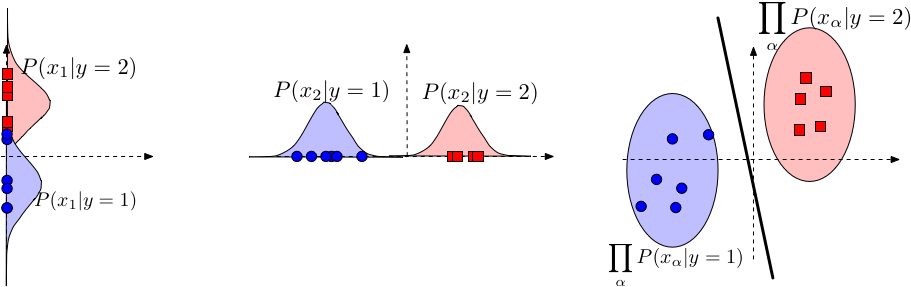
Fig. 23 Naive Bayes leads to a linear decision boundary in many common cases. Illustrated here is the case where \(P\left(x_\alpha \mid y\right)\) is Gaussian and where \(\sigma_{\alpha, c}\) is identical for all \(c\) (but can differ across dimensions \(\alpha\) ). The boundary of the ellipsoids indicate regions of equal probabilities \(P(\mathbf{x} \mid y)\). The red decision line indicates the decision boundary where \(P(y=1 \mid \mathbf{x})=P(y=2 \mid \mathbf{x})\).. Image Credit: CS 4780#
Here \(\alpha\) is just index \(d\).
Suppose that \(y_i \in\{-1,+1\}\) and features are multinomial We can show that
That is,
As before, we define \(P\left(x_\alpha \mid y=+1\right) \propto \theta_{\alpha+}^{x_\alpha}\) and \(P(Y=+1)=\pi_{+}\):
If we use the above to do classification, we can compute for \(\mathbf{w}^{\top} \cdot \mathbf{x}+b\) Simplifying this further leads to
Connection with Logistic Regression#
In the case of continuous features (Gaussian Naive Bayes), when the variance is independent of the class \(\left(\sigma_{\alpha c}\right.\) is identical for all \(c\) ), we can show that
This model is also known as logistic regression. \(N B\) and \(L R\) produce asymptotically the same model if the Naive Bayes assumption holds.
See more proofs below:
https://www.cs.cornell.edu/courses/cs4780/2018fa/lectures/lecturenote05.html.
https://stats.stackexchange.com/questions/142215/how-is-naive-bayes-a-linear-classifier
Section 9.3.4 of Probabilistic Machine Learning: An Introduction.
Time and Space Complexity#
Let \(N\) be the number of training samples, \(D\) be the number of features, and \(K\) be the number of classes.
During training, the time complexity is \(\mathcal{O}(NKD)\) if we are using a brute force approach.
In my implementation,
the main training loop is in _estimate_prior_parameters and _estimate_likelihood_parameters methods.
In the former, we are looping through the classes \(K\) times, but a hidden operation is calculating the
sum of the class counts, which is \(\mathcal{O}(N)\), so the time complexity is \(\mathcal{O}(NK)\), using the
vectorized operation np.sum helps speed up a bit.
In the latter, we are looping through the classes \(K\) times, and for each class, we are looping through
the features \(D\) times, and in each feature loop, we are calculating the mean and variance of the feature,
so the operation of calculating the mean and variance is \(\mathcal{O}(N) + \mathcal{O}(N)\) respectively, bringing the time complexity
to \(\mathcal{O}(2NKD) \approx \mathcal{O}(NKD)\). Even though we are using np.mean and np.var to speed up, the time complexity
for brute force approach is still \(\mathcal{O}(NKD)\).
For the space complexity, we are storing the prior parameters and likelihood parameters, which are of size \(K\) and \(KD\) respectively,
in code, that corresponds to self.pi and self.theta, so the space complexity is \(\mathcal{O}(K + KD) \approx \mathcal{O}(KD)\).
During inference/prediction, the time complexity for predicting one single sample
is \(\mathcal{O}(KD)\), because the predict_one_sample method primarily calls the _calculate_posterior method, which in
turn invokes _calculate_prior and _calculate_joint_likelihood methods, and the time complexity of these two methods
is \(\mathcal{O}(1)\) and \(\mathcal{O}(KD)\) respectively. For _calculate_prior, it just involves us looking up the
self.prior parameter, which is a constant time operation. For _calculate_joint_likelihood, it involves us looping through
the class \(K\) times and looping through the features \(D\) times, so the time complexity is \(\mathcal{O}(KD)\), the mean
and var parameters are now constant time since they are just looked up from self.theta. There is however a np.prod operation
towards the end, but the overall time complexity should still be in the order of \(\mathcal{O}(KD)\).
For the space complexity, besides the stored (not counted) parameters, we are storing the posterior probabilities, which is of size \(K\),
in code, that corresponds to self.posterior, so the space complexity is \(\mathcal{O}(K)\), and if \(K\) is small, then the space complexity
is \(\mathcal{O}(1)\).
Train |
Inference |
|---|---|
\(\mathcal{O}(NKD)\) |
\(\mathcal{O}(KD)\) |
Train |
Inference |
|---|---|
\(\mathcal{O}(KD)\) |
\(\mathcal{O}(1)\) |
References#
Zhang, Aston and Lipton, Zachary C. and Li, Mu and Smola, Alexander J. “Chapter 22.7 Maximum Likelihood.” In Dive into Deep Learning, 2021.
Chan, Stanley H. “Chapter 8.1. Maximum-Likelihood Estimation.” In Introduction to Probability for Data Science, 172-180. Ann Arbor, Michigan: Michigan Publishing Services, 2021
Zhang, Aston and Lipton, Zachary C. and Li, Mu and Smola, Alexander J. “Chapter 22.9 Naive Bayes.” In Dive into Deep Learning, 2021.
Hal Daumé III. “Chapter 9.3. Naive Bayes Models.” In A Course in Machine Learning, January 2017.
Murphy, Kevin P. “Chapter 9.3. Naive Bayes Models.” In Probabilistic Machine Learning: An Introduction. Cambridge (Massachusetts): The MIT Press, 2022.
James, Gareth, Daniela Witten, Trevor Hastie, and Robert Tibshirani. “Chapter 4.4.4. Naive Bayes” In An Introduction to Statistical Learning: With Applications in R. Boston: Springer, 2022.
Mitchell, Tom Michael. Machine Learning. New York: McGraw-Hill, 1997. (His new chapter on Generate and Discriminative Classifiers: Naive Bayes and Logistic Regression)
Jurafsky, Dan, and James H. Martin. “Chapter 4. Naive Bayes and Sentiment Classification” In Speech and Language Processing: An Introduction to Natural Language Processing, Computational Linguistics, and Speech Recognition. Noida: Pearson, 2022.
Bishop, Christopher M. “Chapter 4.2. Probabilistic Generative Models.” In Pattern Recognition and Machine Learning. New York: Springer-Verlag, 2016
- 1
Cite Dive into Deep Learning on this. Also, the joint probability is intractable because the number of parameters to estimate is exponential in the number of features. Use binary bits example, see my notes.
- 2
Not to be confused with the likelihood term \(\mathbb{P}(\mathbf{X} \mid Y)\) in Bayes’ terminology.
- 3
- 4
- 5
Dive into Deep Learning, Section 22.9, this is only assuming that each feature \(\mathbf{x}_d^{(n)}\) is binary, i.e. \(\mathbf{x}_d^{(n)} \in \{0, 1\}\).
- 6
- 7
Probablistic Machine Learning: An Introduction, Section 9.3, pp 328
- 8
- 9
\(\left(\mathbf{X}^{(n)}, Y^{(1)}\right)\) is written as a tuple, when in fact they can be considered 1 single variable.
- 10
Refer to page 470 of [Chan, 2021]. Note that we cannot write it as a product if the data is not independent and identically distributed.
- 11
Cite Kevin Murphy and Bishop.