Implementation
Contents
Implementation#
Utilities#
import sys
from pathlib import Path
parent_dir = str(Path().resolve().parent)
sys.path.append(parent_dir)

import random
import warnings

import matplotlib.pyplot as plt
import numpy as np
import scipy.stats as stats

warnings.filterwarnings("ignore", category=DeprecationWarning)
%matplotlib inline

from utils import seed_all, true_pmf, empirical_pmf
seed_all(42)
Using Seed Number 42
The Setup#
We will use the same setup in Bernoulli Distribution.
Let the true population be defined as a total of \(10000\) people.
We will use the same disease modelling setup.
Let the experiment be a triplet \(\pspace\), this experiment is the action of randomly selecting n people from the true population and subsequently finding out if \(k\) of them have covid. We also emphasize that the process of selecting \(n\) independent and identically distributed people corresponds to selecting \(n\) independent Bernoulli trials, from the same Bernoulli distribution. This means if \(Y \sim \bern(p)\) is the Bernoulli random variable denoting the probability distribution of whether a person has covid or not, then if we repeat this \(Y\) \(n\) number of times independently (drawn with replacement), then we will have a sequence of random variables \(Y_0, Y_1, \ldots, Y_n\), all of which fulfills i.i.d. simply because \(Y_i\) comes from the same distribution \(Y\), and independent because we draw each sample randomly with replacement. Note there should be no ambiguity that \(Y_i\) are copies of the distribution \(Y\), and each copy \(Y_i\) corresponds to the new random draw. The sum \(Y = Y_0 + Y_1 + \ldots + Y_n\), denoted as \(Y\) again (with no confusion with the \(Y\) defined earlier), has a Binomial distribution with parameter \(p\) from the Bernoulli distribution and \(n\) being the number of trials.
Since our problem finding the number of people (\(k\)) who is covid positive out of \(n\) people, we define our sample space to be \(\Omega = \{0, 1, \ldots, n\}\). This is easy to see because out of \(n\) people, with success being 1 and failure being 0, then the sum of these \(n\) trials can at most be \(n = \underbrace{1 + 1 + \ldots + 1}_{\text{n times}}\), at its worst, it can be just \(0\) times. The former is out of \(n\) people, all \(n\) has covid, the latter being out of \(n\) people, none has covid.
Now suppose I want to answer a few simple questions about the experiment. For example, I want to know
What is the probability of 2 people out of \(n=10\) people has covid?
What is the expected value of the true population?
Since we have defined \(Y\) earlier, the corresponding state space \(Y(\S)\) is \(\{0, 1, \ldots, n\}\). We can associate each state \(y \in Y(\S)\) with a probability \(P(Y = y)\). This is the probability mass function (PMF) of \(Y\).
and we seek to find \(p\), and since we already know the true population with \(p=0.2\), we can plot an ideal histogram to see the distribution of how the covid-status of each person in the true population is distributed. An important reminder is that in real world, we often won’t know the true population, and therefore estimating/inferencing the \(p\) parameter becomes important. Also, although there are two parameters, we often will have \(n\) fixed and estimate \(p\).
The PMF (Ideal Histogram)#
# create a true population of 1000 people of 200 1s and 800 0s
true_population = np.zeros(shape=10000)
true_population[:2000] = 1
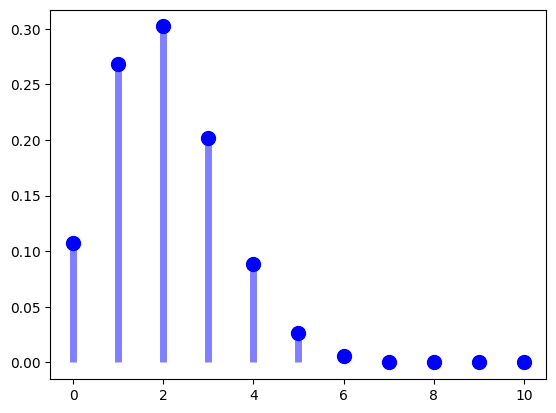
See the plot of PMF for \(p=0.2\) and \(n=10\). This means we are drawing 10 people from the true population in i.i.d. fashion, and the true PMF should be something like the below.
p = 0.2
n = 10
Y = stats.binom(n,p) # the Y ~ Binomial(n, p)
y = np.arange(11) # the states [0, 1, ..., 10]
f = Y.pmf(y) # pmf function
print(f)
plt.plot(y, f, 'bo', ms=10)
plt.vlines(y, 0, f, colors='b', lw=5, alpha=0.5);
[1.07374182e-01 2.68435456e-01 3.01989888e-01 2.01326592e-01
 8.80803840e-02 2.64241152e-02 5.50502400e-03 7.86432000e-04
 7.37280000e-05 4.09600000e-06 1.02400000e-07]
(FIXME): Now I did not use the way in the previous sections because I do not how to plot out this distribution above using the true_population.
But first we must ackowledge this true PMF plotted above is correct.
We can verify by hand that the probability is correct, for example the probability of \(0\) people have covid out of 10 people is like having 10 tails in a row where tails is no covid and heads is covid.
Then it is like
we know this must be true because we know each \(Y_i\) follows a Bernoulli distribution \(Y_i \sim \bern(p=0.2)\) and since these are all independent, by basic probability, then the true probability for this is indeed \(\P(Y_i = T)\) multipled by 10 times.
0.8**10
0.10737418240000006
Y.pmf(0) # verified with hand calculation
0.10737418240000006
If we want to find \(\P \lsq Y = 3 \rsq\), then it is like flipping coin 10 times and get 3 heads out of 10.
Which is 120 cases… since \(10\) choose \(3\) is 120 such cases. And for each case, the probability is \(0.2^{3} \times 0.8^{7}\), so the answer is
120 * (0.2**3 * 0.8 ** 7)
0.2013265920000001
Y.pmf(3)
0.20132659199999992
The true pmf (ideal histogram) gives the answer that out of the true population, if \(n=10\) and \(p=0.2\), the true PMF is realized as:
for y in range(11):
    print(f"PMF for Y={y} is {Y.pmf(y)}")
PMF for Y=0 is 0.10737418240000006
PMF for Y=1 is 0.26843545599999996
PMF for Y=2 is 0.30198988800000004
PMF for Y=3 is 0.20132659199999992
PMF for Y=4 is 0.0880803839999999
PMF for Y=5 is 0.026424115199999983
PMF for Y=6 is 0.005505024000000005
PMF for Y=7 is 0.000786432
PMF for Y=8 is 7.372800000000001e-05
PMF for Y=9 is 4.095999999999997e-06
PMF for Y=10 is 1.0240000000000006e-07
Empirical Distribution (Empirical Histograms)#
sample_100 = np.random.choice(true_population, 100, replace=True)
sample_500 = np.random.choice(true_population, 500, replace=True)
sample_900 = np.random.choice(true_population, 900, replace=True)
def perform_bernoulli_trials(n: int, p: float):
    """
    Perform n Bernoulli trials with success probability p
    and return number of successes. That is to say:
    If I toss coin 10 times, and landed head 7 times, then success rate is
    70% -> this is what I should return. But note this is binary.
    """
    # Initialize number of successes: n_success
    n_success = 0
    rng = np.random.default_rng()

    # Perform trials
    for i in range(n):
        # Choose random number between zero and one: random_number
        random_number = rng.random(size=None)
        # If less than p, it's a success so add one to n_success
        if random_number < p:
            n_success += 1

    return n_success
def perform_bernoulli_trials(population: np.ndarray, n: int, p: float):
    """
    Perform n Bernoulli trials with success probability p
    and return number of successes. That is to say:
    If I toss coin 10 times, and landed head 7 times, then success rate is
    70% -> this is what I should return. But note this is binary.
    """
    # Initialize number of successes: n_success
    n_success = 0

    for i in range(n):
        # Choose random number between zero and one: random_number
        random_number = np.random.choice(population, size=None, replace=True, p=None)
        # If less than p, it's a success so add one to n_success
        if random_number == 1:
            n_success += 1

    return n_success
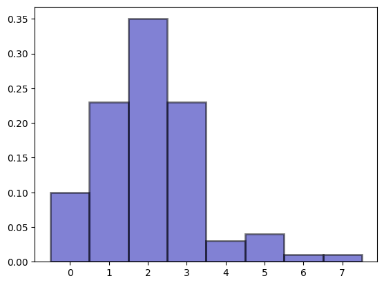
n_repeats = 100
n_covid = np.empty(shape=n_repeats)
for i in range(n_repeats):
    n_covid[i] = perform_bernoulli_trials(true_population, 10, 0.2)
n_covid
array([0., 3., 3., 3., 2., 2., 3., 2., 2., 1., 5., 3., 1., 6., 3., 2., 3.,
       2., 2., 4., 2., 1., 2., 0., 7., 3., 3., 0., 2., 2., 1., 3., 2., 3.,
       1., 2., 1., 2., 1., 1., 1., 2., 2., 3., 3., 2., 3., 2., 1., 2., 3.,
       2., 1., 2., 2., 1., 0., 2., 3., 1., 2., 3., 1., 2., 0., 2., 1., 3.,
       0., 2., 0., 3., 1., 1., 2., 1., 3., 2., 0., 4., 0., 3., 0., 2., 5.,
       2., 2., 3., 5., 3., 1., 1., 1., 2., 5., 2., 4., 1., 1., 2.])
bins = np.arange(0, n_covid.max() + 1.5) - 0.5

plt.hist(
    n_covid,
    bins,
    density=True,
    color="#0504AA",
    alpha=0.5,
    edgecolor="black",
    linewidth=2,
)
(array([0.1 , 0.23, 0.35, 0.23, 0.03, 0.04, 0.01, 0.01]),
 array([-0.5,  0.5,  1.5,  2.5,  3.5,  4.5,  5.5,  6.5,  7.5]),
 <BarContainer object of 8 artists>)
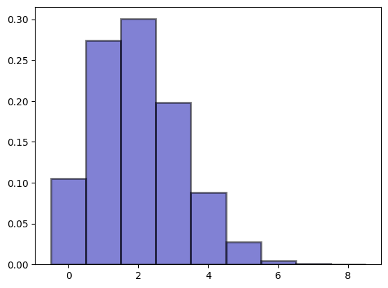
n_repeats = 10000
n_covid = np.empty(shape=n_repeats)
for i in range(n_repeats):
    n_covid[i] = perform_bernoulli_trials(true_population, 10, 0.2)
bins = np.arange(0, n_covid.max() + 1.5) - 0.5
plt.hist(
    n_covid,
    bins,
    density=True,
    color="#0504AA",
    alpha=0.5,
    edgecolor="black",
    linewidth=2,
)
(array([1.054e-01, 2.742e-01, 3.003e-01, 1.985e-01, 8.790e-02, 2.780e-02,
        4.700e-03, 1.100e-03, 1.000e-04]),
 array([-0.5,  0.5,  1.5,  2.5,  3.5,  4.5,  5.5,  6.5,  7.5,  8.5]),
 <BarContainer object of 9 artists>)