Calculus#

See Further Readings for a list of recommended resources if you want to brush up on your calculus.

Integration#

Intuition#

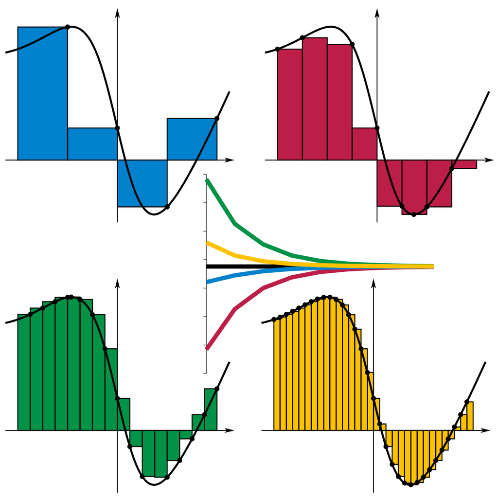
The motivation behind integration is to find the area under a curve. You do this, schematically, by breaking up the interval $[a, b]$ into little regions of width $\Delta x$ and adding up the areas of the resulting rectangles. Here’s an illustration from Wikipedia:

../_images/wiki_1024px-Riemann_sum_convergence.png — Fig. 1 Riemann sum illustration. Image Credit: Wikipedia#

Then we want to make an identification along the lines of

\[\sum_x f(x)\Delta x\approx\int_a^b f(x)\,dx,\]

where we take those rectangle widths to be vanishingly small and refer to them as $dx$.

The symbol used for integration, ∫, is in fact just a stylized “S” for “sum”; The classical definition of the definite integral is $\int_a^b f(x)\,dx=\lim_{\Delta x \to 0} \sum_{x=a}^b f(x)\Delta x$. The limit of the Riemann sum of f(x) between a and b as the increment of X approaches zero (and thus the number of rectangles approaches infinity).

The Fundamental Theorem of Calculus#

Theorem 1 (The Fundamental Theorem of Calculus)

The Fundamental Theorem of Calculus states that for any continuous function $f(x)$ on the closed interval $[a, b]$.

Define $F$ to be a function such that for any $x \in [a, b]$

\[ F(x) = \int_a^x f(t) \, dt \]

Then $F$ is uniformly continuous on $[a, b]$ and and differentiable on the open interval $(a, b)$ and

\[ F^{'}(x) = f(x) = \frac{d}{dx} \int_a^x f(t) \, dt \]

for any $x \in (a, b)$. $F$ is called the antiderivative of $f$.

Corollary 1

The fundamental theorem is often employed to compute the definite integral of a function $f$ for which an antiderivative $F$ is known.

Specifically, if $f$ is a real-valued continuous function on $[a, b]$ and $F$ is an antiderivative of $f$ on $[a, b]$, then

\[ \int_a^b f(x) \, dx = F(b) - F(a) \]

where we assumes that $F$ is continuous on $[a, b]$.

Double Integrals#

See Paul’s Online Notes for a good introduction to double integrals.

Integration and Probability#

Let’s see how to construct measures on a probability space using integration.’ The post below is fully cited from What’s an intuitive explanation for integration?; written by user Felix B.

Integration in probability is often interpreted as “the expected value”. To build up our intuition why, let us start with sums.

Starting Small#

Let’s say you play a game of dice where you win 2€ if you roll a 6 and lose 1€ if you roll any other number. Then we want to calculate what you should expect to receive “on average”. Now most people find the practice of multiplying the payoff by its probability and summing over them relatively straightforward. In this case you get

\[ \text{Expected Payoff} = \frac{1}{6} 2 \text{€} + \frac{5}{6}(-1\text{€}) = -0.5\text{€} \]

Now let us try to formalize this and think about what is happening here. We have a set of possible outcomes $\Omega=\{1,2,3,4,5,6\}$ where each outcome is equally likely. And we have a mapping $Y:\Omega \to \mathbb{R}$ which denotes the payoff. I.e.

\[\begin{split} Y(\omega) = \begin{cases} 2 & \omega = 6,\\ -1 & \text{else} \end{cases} \end{split}\]

And then the expected payoff is $$ \mathbb{E}[Y] = \frac{1}{|\Omega|}\sum_{\omega\in\Omega} Y(\omega) = \frac{1}{6}(2 + (-1) + ... + (-1)) = -0.5 $$

where $|\Omega|$ is the number of elements contained in $\Omega$.

Introducing Infinity#

Now this works fine for finite $\Omega$, but what if the set of possible outcomes is infinite? What if every real number in $[0,1]$ was possible, equally likely, and the payoff would look like this?

\[\begin{split} Y: \begin{cases} [0,1] \to \mathbb{R} \\ \omega \mapsto \begin{cases} 2 & \omega > \frac{5}{6} \\ -1 & \omega \le \frac{5}{6} \end{cases} \end{cases} \end{split}\]

Intuitively this payoff should have the same expected payoff as the previous one. But if we simply try to do the same thing as previously…

\[ \mathbb{E}[Y] = \frac{1}{|\Omega|}\sum_{\omega\in\Omega} Y(\omega) = \frac{1}\infty (\infty - \infty)... \]

Okay so we have to be a bit more clever about this. If we have a look at a plot of your payoff $Y$,

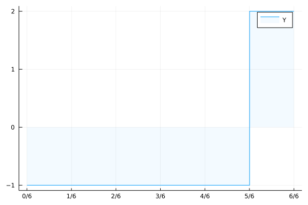
../_images/payoff_plot.png — Fig. 2 Payoff Plot.#

we might notice that the area under the curve is exactly what we want.

\[ -1\text{€}\left(\frac{5}{6}-\frac{0}{6}\right) + 2\text{€} \left(\frac{6}{6} - \frac{5}{6} \right) = -0.5\text{€} \]

Now why is this the same? How are our sums related to an area under a curve?

Summing to one#

To understand this it might be useful to consider what the expected value of a simpler function is

\[\begin{split} \mathbf{1}: \begin{cases} \Omega \to \mathbb{R}\\ \omega \mapsto 1 \end{cases} \end{split}\]

In our first example this was

\[ \frac{1}{|\Omega|} \sum_{\omega\in\Omega} \mathbf{1}(\omega) = \frac{|\Omega|}{|\Omega|} \]

In our second example this would be

\[ \int_{\Omega} 1 d\omega = \int_0^1 1 d\omega \]

Now if we recall how the integral (area under the curve) is calculated we might notice that in case of indicator functions, we are weighting the height of the indicator function with the size of the interval. And the size of the interval is its length.

Similarly we could move $\frac{1}{|\Omega|}$ into the sum and view it as the weighting of each $\omega$. And here is where we have the crucial difference:

In the first case individual $\omega$ have a weight (a probability), while individual points in an interval have no length/weight/probability. But while sets of individual points have no length, an infinite union of points with no length/probability can have positive length/probability.

This is why probability is closely intertwined with measure theory, where a measure is a function assigning sets (e.g. intervals) a weight (e.g. lenght, or probability).

Doing it properly#

So if we restart our attempt at defining the expected value, we start with a probability space $\Omega$ and a probability measure $P$ which assigns subsets of $\Omega$ a probability. A real valued random variable (e.g. payoff) $Y$ is a function from $\Omega$ to $\mathbb{R}$. And if it only takes a finite number of values in $\mathbb{R}$ (i.e. $Y(\Omega)\subseteq \mathbb{R}$ is finite), then we can calculate the expected value by going through these values, weightening them by the probability of their preimages and summing them.

\[ \mathbb{E}[Y] = \sum_{y\in Y(\Omega)} y P[Y^{-1}(\{y\})] \]

To make notation more readable we can define

\[\begin{split} \begin{aligned} P[Y\in A] &:= P[Y^{-1}(A)] \qquad\text{and} \\ P[Y=y]&:=P[Y\in\{y\}] \end{aligned} \end{split}\]

In our finite example the expected value is

\[\begin{split} \begin{aligned} \mathbb{E}[Y] &= 2 P(Y=2) + (-1) P(Y=-1)\\ &=2 P(Y^{-1}[\{2\}]) +(-1)P(\{1,2,3,4,5\})\\ &= 2 \frac16 -1 \frac56 = -0.5 \end{aligned} \end{split}\]

In our infinite example the expected value is

\[\begin{split} \begin{aligned} \mathbb{E}[Y] &= 2P(Y=2) + (-1)P(Y=-1)\\ &= 2P\left(\left(\frac56, 1\right]\right) - P\left(\left[0, \frac56\right]\right) = \int_0^1 Y d\omega\\ &= 2 \frac16 - \frac56 = -0.5 \end{aligned} \end{split}\]

Now it turns out that you can approximate every $Y$ with infinite image $Y(\Omega)$ with a sequence of mappings $Y_n$ with finite image. And that the limit

\[ \int_\Omega Y dP := \lim_n \int_\Omega Y_n dP := \sum_{y\in Y_n(\Omega)} y P(Y=y) \]

is also well defined and independent of the sequence $Y_n$.

Lebesgue Integral#

The integral we defined above is called the Lebesgue Integral. The neat thing about it is, that

Riemann integration is a special case of it, if we integrate over the Lebesgue Measure $\lambda$ which assigns intervals $[a,b]$ their length $\lambda([a,b])=b-a$.

\[ \int_{[a,b]} f d\lambda = \int_a^b f(x) dx \]

Sums and series are also a special case using sequences $(a(n), n\in\mathbb{N})$ and a “counting measure” $\mu$ on $\mathbb{N}$ which assigns a set $A$ its size $\mu(A) = |A|$. Then

\[ \int_{\Omega} a d\mu = \sum_{n\in\mathbb{N}} a(n) \]

The implications are of course for one, that one can often treat integration and summation interchangeably. Proving statements for Lebesgue integrals is rarely harder than proving them for Riemann integrals and in the first case all results also apply to series and sums.

It also means we can properly deal with “mixed cases” where some individual points have positive probability and some points have zero probability on their own but sets of them have positive probability.

My stochastics professor likes to call integration just “infinite summation” because in some sense you are just summing over an infinite number of elements in a “proper way”.

The lebesgue integral also makes certain real functions integrable which are not integrable with riemann integration. The function $\mathbf{1}_{\mathbb{Q}}$ is not riemann integrable, but poses no problem for lebesgue integration. The reason is, that riemann integration subdivides the $x$-axis and $y$-axis into intervals without consulting the function that is supposed to be integrated, while lebesgue integration only subdivides the $y$-axis and utilizes the preimage information about the function that is supposed to be integrated.

Back to Intuition#

Now the end result might not resemble our intuition about “expected values” anymore. We get some of that back with theorems like the law of large numbers which proves that averages

\[\frac{1}{n} \sum_{k=1}^n X_k\]

of independently, identically distributed random variables converge (in various senses) to the theoretically defined expected value $\mathbb{E}[X]$.

A note on Random Variables#

In our examples above, only the payoff $Y$ was a random variable (a function from the probability space $\Omega$ to $\mathbb{R}$). But since we can compose functions by chaining them, nothing would have stopped us from defining the possible die faces as a random variable of some unknown probability space $\Omega$. Since our payoff is just a function of the die faces, their composition would also be a function from $\Omega$. And it is often convenient not to define $\Omega$ and start with random variables right away, as it allows easy extensions of our models without having to redefine our probability space. Because we treat the underlying probability space as unknown anyway and only work with known windows (random variables) into it. Notice how you could not discern the die faces $\{1,...,5\}$ from payoff $Y=-1$ alone. So random variables can also be viewed as information filters.

Lies#

While we would like our measures to assign every subset of $\Omega$ a number, this is generally not possible without sacrificing its usefulness.

If we wanted a measure on $\mathbb{R}$ which fulfills the following properties

translation invariance (moving a set about does not change its size)
countable summability of disjoint sets
positive
finite on every bounded set

we are only left with the $0$ measure (assigning every set measure 0).

Proofsketch: Use the axiom of choice to select a representative of every equivalence class of the equivalence relation $x-y\in \mathbb{Q}$ on the set $[0,1]$. This set of representatives is not measurable, because translations by rational numbers modulo 1 transforms it into distinct other representation sets of the equivalence relation. And since they are disjoint and countable we can sum over them and get the measure of the entire interval $[0,1]$. But an infinite sum of equally sized sets can not be finite if they are not all $0$. Therefore the set $[0,1]$ must have measure 0 and by translation and summation all other sets in $\mathbb{R}$

For this reason we have to restrict ourselves to a set of “measurable sets” (a sigma Algebra) which is only a subset of the powerset $\mathcal{P}(\Omega)$ of $\Omega$. This conundrum also limits the functions we can integrate with lebesgue integration to the set of “measurable functions”.

But all of these things are technicalities distracting from the intuition.

Probability & Statistics

Calculus

Contents