Concept

Conditional Expectation

Definition 79 (Conditional Expectation)

The conditional expectation of \(X\) given \(Y=y\) is

\[ \mathbb{E}[X \mid Y=y]=\sum_x x p_{X \mid Y}(x \mid y) \]

for discrete random variables, and

\[ \mathbb{E}[X \mid Y=y]=\int_{-\infty}^{\infty} x f_{X \mid Y}(x \mid y) d x \]

for continuous random variables.

Remark 14 (Conditional Expectation is the Expectation for a Sub-Population)

Similar to Remark 13, we need to be clear that the conditional expectation is the expectation for a sub-population. In particular, the expectation of \(\mathbb{E}[X \mid Y=y]\) is taken with respect to \(f_{X \mid Y}(x \mid y)\), and this means that the random variable \(Y\) is already fixed at the state \(Y=y\). Consequently, \(Y\) is no longer random, the only source of randomness is \(X\). However the expression is a function of \(Y\). This may be confusing since earlier sections say the conditional distribution of \(X\) given \(Y\) is a distribution for a sub-population in \(X\). See here and here for examples.

Less formally, we can say that the conditional distribution (PDF) of a random variable \(X\) given a specific state \(Y=y\) can be loosely considered a function of \(X\). Furthermore, when you take the expectation of \(X \mid Y=y\) for a specific state \(Y=y\), you get back a number. This number however is dependent on the state \(Y=y\) that you have chosen. Therefore the conditional expectation \(\mathbb{E}[X \mid Y=y]\) gives you a number, but \(\mathbb{E}[X \mid Y]\) gives you a function where \(Y\) is allowed to vary. Since \(Y\) is a random variable, the function \(\mathbb{E}[X \mid Y]\) is also a random variable.

See here for a more rigourous treatment in terms of measure theory.

However, do note that in earlier chapters on Expectation, we have seen that the expectation in itself is deterministic, as it represents the population mean.

The Law of Total Expectation

Just like the Law of Total Probability stated in Theorem 3, we can also state a similar law for the expectation.

Theorem 28 (Law of Total Expectation)

Let \(X\) and \(Y\) be random variables. Let \(\P\) be a probability function defined over the probability space \(\pspace\).

Let \(\{A_1, \ldots, A_n\}\) be a partition of the sample space \(\Omega_Y\). This means that \(A_1, \ldots, A_n\) are disjoint and \(\Omega_Y = A_1 \cup \cdots \cup A_n\). Then, for any \(X\), we have

\[ \mathbb{E}[X] = \sum_{i=1}^{n} \mathbb{E}[X \mid Y \in A_i] \P(A_i) \]

where \(\P(A_i)\) is the probability of \(Y\) being in \(A_i\).

More formally stated,

\[ \mathbb{E}[X] = \sum_{y} \mathbb{E}[X \mid Y=y] p_Y(y) \]

for the discrete case, and

\[ \mathbb{E}[X] = \int_{y} \mathbb{E}[X \mid Y=y] f_Y(y) dy \]

for the continuous case.

An enlightening figure below extracted from [Chan, 2021] illustrates the Law of Total Expectation for the discrete case.

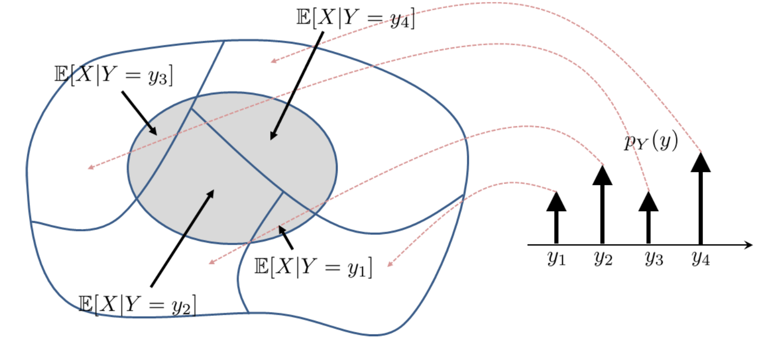
Fig. 10 Decomposing the expectation \(\mathbb{E}[X]\) into “sub-expectations” \(\mathbb{E}[X \mid Y=y]\).

Corollary 11 (The Law of Iterated Expectation)

Let \(X\) and \(Y\) be random variables, then we have

(35)\[ \mathbb{E}[X] = \mathbb{E}_{Y}[\mathbb{E}_{X \mid Y}[X]] \]

Proof. We can use the Law of Total Expectation to prove this corollary.

Define \(\mathbb{E}[X] = \sum_{y} \mathbb{E}[X \mid Y=y] p_Y(y)\). Then further treat \(\mathbb{E}[X \mid Y=y]\) as a function of \(Y\),

\[ g(Y) = \mathbb{E}[X \mid Y=y] \]

then we write

\[\begin{split} \begin{aligned} \mathbb{E}[X] &= \sum_{y} \mathbb{E}[X \mid Y=y] p_Y(y) \\ &= \sum_{y} g(Y) p_Y(y) \\ &= \mathbb{E}_{Y}[g(Y)] \\ &= \mathbb{E}_{Y}[\mathbb{E}_{X \mid Y}[X]] \end{aligned} \end{split}\]

Conditional Variance

Similarly, we can define the conditional variance of \(X\) given \(Y=y\) as follows.

Definition 80 (Conditional Variance)

Let \(X\) and \(Y\) be random variables, then the conditional variance of \(X\) given \(Y=y\) is defined as

\[\begin{split} \begin{aligned} \text{Var}[X \mid Y=y] &= \mathbb{E}[X^2 \mid Y=y] - \mathbb{E}[X \mid Y=y]^2 \\ \end{aligned} \end{split}\]