The Geometry of Multivariate Gaussians
Contents
The Geometry of Multivariate Gaussians#
By the eigendecomposition theorem, we can write the covariance matrix \(\boldsymbol{\Sigma}\) as:
where \(\boldsymbol{u}_d\) is the \(d\)th eigenvector of \(\boldsymbol{\Sigma}\) and \(\lambda_d\) is the corresponding eigenvalue. The eigenvectors are orthogonal, so \(\boldsymbol{U}^{T} \boldsymbol{U} = \boldsymbol{I}\).
The geometry of a multivariate Gaussian distribution is defined by its covariance matrix, which can be represented in terms of its eigenvalues and eigenvectors. The eigenvalues represent the magnitude of the variance along each eigenvector (principal axis) and determine the shape of the ellipsoid that characterizes the distribution. The eigenvectors define the orientation of the principal axes and hence the orientation of the ellipsoid. This information allows us to perform various operations such as transforming the coordinates of the data points, projecting the data onto a lower-dimensional subspace, or rotating the ellipsoid to align with the coordinate axes.
This is true, but it is not immediately obvious why. Let’s see why.
First, we have established that the covariance matrix can be decomposed to a matrix of eigenvectors and a diagonal matrix of eigenvalues. We claim that for each dimension \(d\), the variance of the \(d\)th dimension is given by \(\lambda_d\), and the direction of the \(d\)th dimension is given by \(\boldsymbol{u}_d\).
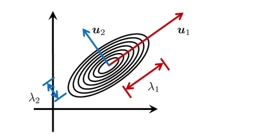
Fig. 12 The shape of multivariate gaussian is defined by its mean and covariance. Image Credit: [Chan, 2021].#
Why Eigenvalues and Eigenvectors defined the shape of Multivariate Gaussian?#
Consider a random vector \(\mathbf{X} \in \mathbb{R}^D\) with mean vector \(\boldsymbol{\mu}\) and covariance matrix \(\boldsymbol{\Sigma}\). The probability density function of the multivariate Gaussian distribution is given by:
where \(|\boldsymbol{\Sigma}|\) is the determinant of \(\boldsymbol{\Sigma} \).
The level sets (see contours) of the Gaussian distribution correspond to the set of points in the \(D\)-dimensional space that have the same probability density. The level set at a given level \(\lambda\) is given by the equation:
where \(\lambda\) is a constant. Rearranging, we get:
So we have rearranged such that the right-hand side is a constant, and we represent it by \(\lambda^{'}\). Why can we do this? That is because in multivariate gaussian, you observed that only the exponential term is dependent on \(\boldsymbol{x}\), and therefore, we might as well use the simplified term above to represent the level set of the multivariate gaussian. It is merely a change of variable.
We claim that the level set of the multivariate Gaussian distribution, defined by:
is an ellipse in the \(D\)-dimensional space.
To see why the equation defines an ellipse, we can use the eigendecomposition of the covariance matrix. Let \(\Sigma = Q \Lambda Q^T\) be the eigendecomposition, where \(Q\) is an orthogonal matrix of eigenvectors and \(\Lambda\) is a diagonal matrix of eigenvalues. Substituting this into the equation, we get:
Let \(Y = Q^T (X - \mu)\). Then, the equation becomes:
This equation represents a set of ellipses in the Y space, where the eigenvectors of \(\Lambda^{-1}\) are the principal axes of the ellipses and the eigenvalues of \(\Lambda^{-1}\) are the reciprocals of the variances along the principal axes. The ellipses in the Y space can be transformed back into the X space by multiplying by \(Q\).
Thus, we have shown that the level sets of a multivariate Gaussian distribution are ellipsoids centered at the mean vector and defined by the covariance matrix, which in turn is defined by the principal axes and variances of the distribution (eigenvalues and eigenvectors of the covariance matrix).
Remark 17 (Remark)
So indeed, the shape of the level set of the multivariate Gaussian distribution is an ellipse. In an ellipse, there is the notion of a major axis and a minor axis. The major axis is the axis that is longer than the minor axis. The major axis is the axis along which the distribution has the largest variance. And by the reasoning we have just done, we see that the major axis of a multivariate Gaussian is the eigenvector of the covariance matrix that corresponds to the largest eigenvalue.
Further Readings#
Bishop, Christopher M. “Chapter 2.3. The Gaussian Distribution.” In Pattern Recognition and Machine Learning. New York: Springer-Verlag, 2016
Why probability contours for the multivariate Gaussian are elliptical
Why are contours of a multivariate Gaussian distribution elliptical?