Probability Inequalities#

In this section, we will only list the definitions of the various inequalities without proofs. We will prove them along the way in the next section.

This section is mainly adapted from [Chan, 2021].

Union Bound#

Theorem 46 (Union Bound)

The first inequality is the union bound we had introduced when we discussed the axioms of probabilities. The union bound states the following:

Let \(A_{1}, \ldots, A_{N}\) be a collection of sets. Then

\[ \mathbb{P}\left[\bigcup_{n=1}^{N} A_{n}\right] \leq \sum_{n=1}^{N} \mathbb{P}\left[A_{n}\right] \]

Remark 18 (Tightness of the Union Bound)

Remark. The tightness of the union bound depends on the amount of overlapping between the events \(A_{1}, \ldots, A_{n}\), as illustrated in Fig. 13. If the events are disjoint, the union bound is tight. If the events are overlapping significantly, the union is loose. The idea of the union bound is the principle of divide and conquer. We decompose the system into smaller events for a system of \(n\) variables and use the union bound to upper-limit the overall probability. If the probability of each event is small, the union bound tells us that the overall probability of the system will also be small [Chan, 2021].

../../_images/chan_fig6.4.jpeg — Fig. 13 Conditions under which the union bound is loose or tight. [Left] The union bound is loose when the sets are overlapping. [Right] The union bound is tight when the sets are (nearly) disjoint. Image Credit: [Chan, 2021].#

The Cauchy-Schwarz Inequality#

Theorem 47 (Cauchy-Schwarz Inequality)

Let \(X\) and \(Y\) be two random variables. Then

\[ \mathbb{E}[X Y]^{2} \leq \mathbb{E}\left[X^{2}\right] \mathbb{E}\left[Y^{2}\right] \]

Remark 19 (Application of the Cauchy-Schwarz Inequality)

The Cauchy-Schwarz inequality is useful in analyzing \(\mathbb{E}[X Y]\). For example, we can use the Cauchy-Schwarz inequality to prove that the correlation coefficient \(\rho\) is bounded between \(-1\) and 1.

Jensen’s Inequality#

Our next inequality is Jensen’s inequality. To motivate the inequality, we recall that

\[ \operatorname{Var}[X]=\mathbb{E}\left[X^{2}\right]-\mathbb{E}[X]^{2} \]

Since \(\operatorname{Var}[X] \geq 0\) for any \(X\), it follows that

\[ \underbrace{\mathbb{E}\left[X^{2}\right]}_{=\mathbb{E}[g(X)]} \geq \underbrace{\mathbb{E}[X]^{2}}_{=g(\mathbb{E}[X])} . \]

Jensen’s inequality is a generalization of the above result by recognizing that the inequality does not only hold for the function \(g(X)=X^{2}\) but also for any convex function \(g\). The theorem is stated as follows:

Theorem 48 (Jensen’s Inequality)

Let \(X\) be a random variable, and let \(g: \mathbb{R} \rightarrow \mathbb{R}\) be a convex function. Then

\[ \mathbb{E}[g(X)] \geq g(\mathbb{E}[X]) \]

Remark 20 (Convex and Concave Functions)

If the function \(g\) is concave, then the inequality sign is flipped: \(\mathbb{E}[g(X)] \leq g(\mathbb{E}[X])\). The way to remember this result is to remember that \(\mathbb{E}\left[X^{2}\right]-\mathbb{E}[X]^{2}=\operatorname{Var}[X] \geq 0\).

Now, what is a convex function? Informally, a function \(g\) is convex if, when we pick any two points on the function and connect them with a straight line, the line will be above the function for that segment. This definition is illustrated in Figure 6.5 Consider an interval \([x, y]\), and the line segment connecting \(g(x)\) and \(g(y)\). If the function \(g(\cdot)\) is convex, then the entire line segment should be above the curve.

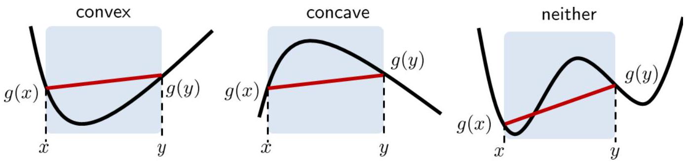
../../_images/chan_fig6.5.jpeg — Fig. 14 Illustration of a convex function, a concave function, and a function that is neither convex nor concave. Image Credit: [Chan, 2021].#

Definition 101 (Convex)

A function \(g\) is convex if

\[ g(\lambda x+(1-\lambda) y) \leq \lambda g(x)+(1-\lambda) g(y) \]

for any \(0 \leq \lambda \leq 1\)

Here \(\lambda\) represents a “sweeping” constant that goes from \(x\) to \(y\). When \(\lambda=1\) then \(\lambda x+(1-\lambda) y\) simplifies to \(x\), and when \(\lambda=0\) then \(\lambda x+(1-\lambda) y\) simplifies to \(y\).

For a more formal treatment with examples, see [Chan, 2021].

Markov’s Inequality#

Our next inequality, Markov’s inequality, is an elementary inequality that links probability and expectation.

Theorem 49 (Markov’s Inequality)

Let \(X \geq 0\) be a non-negative random variable. Then, for any \(\varepsilon>0\), we have

\[ \mathbb{P}[X \geq \varepsilon] \leq \frac{\mathbb{E}[X]}{\varepsilon} \]

For a more formal treatment with examples, see [Chan, 2021].

Chebyshev’s Inequality#

The next inequality is a simple extension of Markov’s inequality. The result is known as Chebyshev’s inequality.

Theorem 50 (Chebyshev’s Inequality)

Let \(X\) be a random variable with mean \(\mu\). Then for any \(\varepsilon>0\) we have

\[ \mathbb{P}[|X-\mu| \geq \varepsilon] \leq \frac{\operatorname{Var}[X]}{\varepsilon^{2}} \]

Corollary 14 (Chebyshev’s Inequality for i.i.d. Random Variables)

Let \(X_{1}, \ldots, X_{N}\) be i.i.d. random variables with mean \(\mathbb{E}\left[X_{n}\right]=\mu\) and variance \(\operatorname{Var}\left[X_{n}\right]=\sigma^{2}\). Let \(\bar{X}=\frac{1}{N} \sum_{n=1}^{N} X_{n}\) be the sample mean. Then

\[ \mathbb{P}\left[\left|\bar{X}-\mu\right|>\epsilon\right] \leq \frac{\sigma^{2}}{N \epsilon^{2}} . \]

Chernoff’s Bound#

We now introduce a powerful inequality or a set of general procedures that gives us some highly useful inequalities. The idea is named for Herman Chernoff, although it was actually due to his colleague Herman Rubin.

Theorem 51 (Chernoff’s Bound)

Let \(X\) be a random variable. Then, for any \(\varepsilon \geq 0\), we have that

\[ \mathbb{P}[X \geq \varepsilon] \leq e^{-\varphi(\varepsilon)}, \]

where

\[ \varphi(\varepsilon)=\max _{s>0}\left\{s \varepsilon-\log M_{X}(s)\right\}, \]

and \(M_{X}(s)\) is the moment-generating function.

Application of Chernoff and Chebyshev’s Inequality#

See section 6.2.7 of [Chan, 2021] for more details.

Hoeffding’s Inequality#

Chernoff’s bound can be used to derive many powerful inequalities, one of which is Hoeffding’s inequality. This equality is the basis of Machine Learning’s PACE (Probably Approximately Correct) framework and the VC dimension.

Theorem 52 (Hoeffding’s Inequality)

Let \(X_{1}, \ldots, X_{N}\) be i.i.d. random variables with \(0 \leq X_{n} \leq 1\), and \(\mathbb{E}\left[X_{n}\right]=\mu\). Then

\[ \mathbb{P}\left[\left|\bar{X} - \mu\right|>\epsilon\right] \leq 2 e^{-2 \epsilon^{2} N}, \]

where \(\bar{X} = \frac{1}{N} \sum_{n=1}^{N} X_{n}\)

Proof. See [Chan, 2021] for the proof.

Lemma 1 (Hoeffding’s Lemma)

Let \(a \leq X \leq b\) be a random variable with \(\mathbb{E}[X]=0\). Then

\[ M_{X}(s) \stackrel{\text { def }}{=} \mathbb{E}\left[e^{s X}\right] \leq \exp \left\{\frac{s^{2}(b-a)^{2}}{8}\right\} . \]

Proof. See [Chan, 2021] for the proof.

Interpretation of Hoeffding’s Inequality#

This section is extracted verbatim from Chan, Stanley H. “Chapter 6.2.8. Hoeffding’s inequality.” In Introduction to Probability for Data Science. Ann Arbor, Michigan: Michigan Publishing Services, 2021.

Interpreting Hoeffding’s inequality. One way to interpret Hoeffding’s inequality is to write the equation as

\[ \mathbb{P}\left[\left|\bar{X}-\mu\right|>\epsilon\right] \leq \underbrace{2 e^{-2 \epsilon^{2} N}}_{\delta}, \]

which is equivalent to

\[ \mathbb{P}\left[\left|\bar{X}-\mu\right| \leq \epsilon\right] \geq 1-\delta . \]

This means that with a probability at least \(1-\delta\), we have

\[ \bar{X}-\epsilon \leq \mu \leq \bar{X}+\epsilon . \]

If we let \(\delta=2 e^{-2 \epsilon^{2} N}\), this becomes

\[ \bar{X}-\sqrt{\frac{1}{2 N} \log \frac{2}{\delta}} \leq \mu \leq \bar{X}+\sqrt{\frac{1}{2 N} \log \frac{2}{\delta}} . \]

This inequality is a confidence interval (see Chapter 9). It says that with probability at least \(1-\delta\), the interval \(\left[\bar{X}-\epsilon, \bar{X}+\epsilon\right]\) includes the true population mean \(\mu\).

There are two questions one can ask about the confidence interval:

Given \(N\) and \(\delta\), what is the confidence interval? Equation \(6.28\) tells us that if we know \(N\), to achieve a probability of at least \(1-\delta\) the confidence interval will follow Equation 6.28. For example, if \(N=10,000\) and \(\delta=0.01, \sqrt{\frac{1}{2 N} \log \frac{2}{\delta}}=0.016\). Therefore, with a probability at least \(99 \%\), the true population mean \(\mu\) will be included in the interval

\[ \bar{X}-0.16 \leq \mu \leq \bar{X}+0.16 \text {. } \]

If we want to achieve a certain confidence interval, what is the \(N\) we need? If we are given \(\epsilon\) and \(\delta\), the \(N\) we need is

\[ \delta \leq 2 e^{-2 \epsilon^{2} N} \quad \Rightarrow \quad N \geq \frac{\log \frac{2}{\delta}}{2 \epsilon^{2}} . \]

For example, if \(\delta=0.01\) and \(\epsilon=0.01\), the \(N\) we need is \(N \geq 26,500\).

When is Hoeffding’s inequality used? Hoeffding’s inequality is fundamental in modern machine learning theory. In this field, one often wants to quantify how well a learning algorithm performs with respect to the complexity of the model and the number of training samples. For example, if we choose a complex model, we should expect to use more training samples or overfit otherwise. Hoeffding’s inequality provides an asymptotic description of the training error, testing error, and the number of training samples. The inequality is often used to compare the theoretical performance limit of one model versus another model. Therefore, although we do not need to use Hoeffding’s inequality in this book, we hope you appreciate its tightness.

Probability & Statistics

Probability Inequalities

Contents