Concept

This topic is quite theoretical and heavy. I do not have the ability to explain them in an intuitive way. Therefore, most of the content here is adapted from the following sources:

• ECE595: Learning Theory

• Mostafa Samir: Machine Learning Theory

• Zhang Wei: Learning Theory

Therefore, this section serves as a document/reference and all credits go to the authors of the above sources.

Some Abuse of Notations

Remark 27 (Notations)

We will abbrieviate:

$${\mathcal{R}}_{\mathcal{D}}\{\mathcal{L}((\mathbf{x},y),h)\}:={\mathcal{R}}_{\mathcal{D}}\left\{h\right\}$$

$${\mathbb{P}}_{\mathcal{D}}:=\mathcal{D}$$

when the context is clear.

The author used $g$ as the final hypothesis learnt by the algorithm, we will however use $h_S$ to denote $g$. Therefore, some images from the author will have $g$ instead of $h_S$.

Problem Statement

When we have built a classifier, one question people always ask is how good the classifier is. They want to evaluate the classifier. They want to see whether the classifier is able to predict what it is supposed to predict. Often times, the “gold standard” is to report the classification accuracy: Give me a testing dataset, and I will tell you how many times the classifier has done correctly. This is one way of evaluating the classifier. However, does this evaluation method really tells us how good the classifier is? Not clear. All it says is that for this classifier trained on a particular training dataset and tested on a particular testing dataset, the classifier performs such and such. Will it perform well if we train the classifier using another training set, maybe containing more data points? Will it perform well if we test it on a different testing dataset? It seems that we lack a way to quantify the generalization ability of our classifier.

There is another difficulty. When we train the classifier, we can only access the training data but not the testing data. This is like taking an exam. We can never see the exam questions when we study, for otherwise we will defeat the purpose of the exam! Since we only have the training set when we design our classifier, how do we tell whether we have trained a good classifier? Should we choose a more complex model? How many samples do we need? Remember, we cannot use any testing data and so all the evaluation has to be done internally using the training data. How to do that? Again, we are missing a way to quantify the performance of the classifier.

The objective of this chapter is to answer a few theoretical (and also practical) questions in learning:

1. Is learning feasible?

2. How much can a classifier generalize?

3. What is the relationship between number of training samples and the complexity of the classifier?

4. How do we tell whether we have obtained a good classifier during the training?

Notations

Let’s refresh ourselves with some notations.

We have a training dataset $\mathcal{S}$ sampled $\mathbf{\text{i.i.d.}}$ from the underlying and unknown distribution $\mathcal{D}$.

$$\mathcal{S}=\{({\mathbf{x}}^{(1)},y^{(1)}),({\mathbf{x}}^{(2)},y^{(2)}),\dots ,({\mathbf{x}}^{(N)},y^{(N)})\}\stackrel{\text{iid}}{\sim }\mathcal{D}$$

where ${\mathbf{x}}^{(n)}\in {\mathbb{R}}^D$ is the input vector and $y^{(n)}\in \mathcal{Y}$ is the corresponding label. We call ${\mathbf{x}}^{(n)}$ the $n$-th input vector and $y^{(n)}$ the $n$-th label. We call $\mathcal{S}$ the training dataset. We call $\mathcal{D}$ (${\mathbb{P}}_{\mathcal{D}}$) the underlying distribution.

Now there is an unknown target function $f:\mathcal{X}\to \mathcal{Y}$1 which maps $\mathbf{x}$ to a label $y=f(\mathbf{x})$. The set $\mathcal{X}$ contains all the input vectors, and we call $\mathcal{X}$ the input space. The set $\mathcal{Y}$ contains the corresponding labels, and we call $\mathcal{Y}$ the output space.

In any supervised learning scenario, there is always a training set $\mathcal{S}$ sampled from ${\mathbb{P}}_{\mathcal{D}}$. The training set contains $N$ input-output pairs $({\mathbf{x}}^{(1)},y^{(1)}),\dots ,({\mathbf{x}}^{(N)},y^{(N)})$, where ${\mathbf{x}}^{(n)}$ and $y^{(n)}$ are related via $y^{(n)}=$ $f\left({\mathbf{x}}^{(n)}\right)$, for $n=1,\dots ,N$. These input-output pairs are called the data points or samples. Since $\mathcal{S}$ is a finite collection of data points, there are many $\mathbf{x}\in \mathcal{X}$ that do not live in the training set $\mathcal{S}$. A data point ${\mathbf{x}}^{(n)}$ that is inside $\mathcal{S}$ is called an in-sample, and a data point $\mathbf{x}$ that is outside $\mathcal{S}$ is called an out-sample.

When we say that we use a machine learning algorithm to learn a classifier, we mean that we have an algorithmic procedure $\mathcal{A}$ (i.e. Logistic Regression, KNN etc) which uses the training set $\mathcal{S}$ to select a hypothesis function $h_S:\mathcal{X}\to \mathcal{Y}$. The hypothesis function is again a mapping from $\mathcal{X}$ to $\mathcal{Y}$, because it tells what a sample $\mathbf{x}$ is being classified. However, a hypothesis function $h_S$ learned by the algorithm is not the same as the target function $f$. We never know $f$ because $f$ is simply unknown. No matter how much we learn, the hypothesis function $h_S$ is at best an approximation of $f$. The approximation error can be zero in some hand-craved toy examples, but in general $h_S\ne f$. All hypothesis functions are contained in the hypothesis set $\mathcal{H}$. If the hypothesis set is finite, then $\mathcal{H}=\{h_1,\dots ,h_M\}$, and $h_S$ will be one of these $h_m$ ‘s. A hypothesis set can be infinite, for example we can perturb a perceptron decision boundary by an infinitesimal step to an infinite hypothesis set. An infinite hypothesis set is denoted by $\mathcal{H}=\left\{h_{\sigma }\right\}$, where $\sigma$ denotes a continuous parameter.

The drawings in Fig. 15 illustrate a few key concepts we just mentioned. On the left hand side there is an input space $\mathcal{X}$, which contains a small subset $\mathcal{S}$. The subset $\mathcal{S}$ is the training set, which includes a finite number of training samples or in-samples. There is an unknown target function $f$. The target function $f$ maps an ${\mathbf{x}}^{(n)}$ to produce an output $y^{(n)}=f\left({\mathbf{x}}^{(n)}\right)$, hence giving a colored dots in the middle of the figure. The objective of learning is to learn a classifier which can classify the red from the blue. The space containing all the possible hypothesis is the hypothesis set $\mathcal{H}$, which contains $h_1,\dots ,h_M$. The final hypothesis function returned by the learning algorithm is $h_S$.

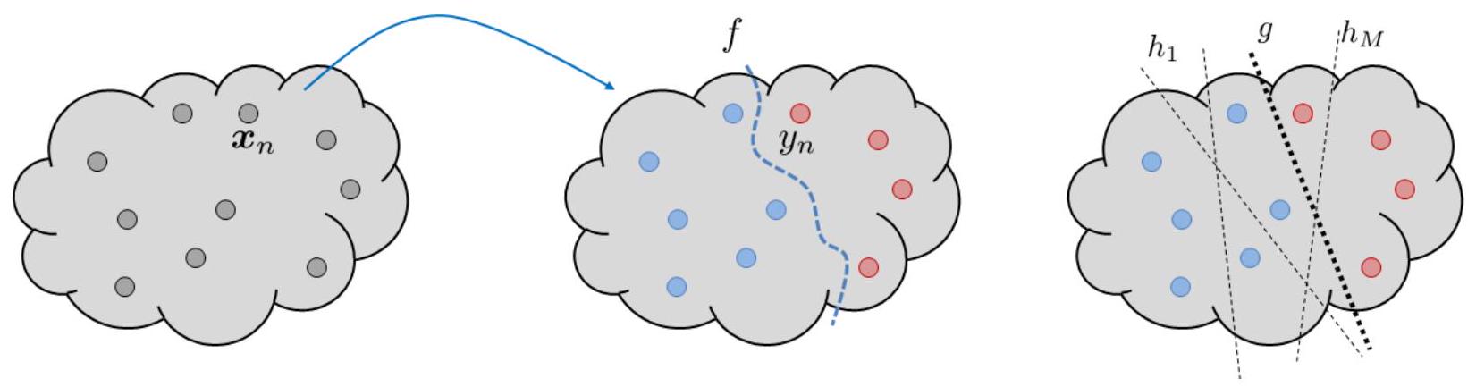
Fig. 15 [Left] Treat the cloud as the entire input space $\mathcal{X}$ and correspondingly the output space $\mathcal{Y}$. The dots are the in-samples ${\mathbf{x}}^{(1)},\dots ,{\mathbf{x}}^{(N)}$. The target function is a mapping $f$ which takes ${\mathbf{x}}^{(n)}$ and send it to $y^{(n)}$. The red and blue colors indicate the class label. [Right] A learning algorithm picks a hypothesis function $h_S$ from the hypothesis set $\mathcal{H}=\{h_1,\dots ,h_M\}$. Note that some hypotheses are good, and some are bad. A good learning algorithm will pick a good hypothesis, and a bad learning algorithm can pick a bad hypothesis.

Fig. 16 illustrates what we called a probabilistic learning model. It is called a probabilistic learning model because there is an unknown distribution $p(\mathbf{x})$. The training samples $\{{\mathbf{x}}^{(1)},\dots ,{\mathbf{x}}^{(N)}\}$ are generated according to ${\mathbb{P}}_{\mathcal{D}}(\mathbf{x})$. The same ${\mathbb{P}}_{\mathcal{D}}(\mathbf{x})$ also generates the testing samples $\mathbf{x}$. It is possible to lift the probabilistic assumption so that the training samples are drawn deterministically. In this case, the samples are simply fixed set of data points $\{{\mathbf{x}}^{(1)},\dots ,{\mathbf{x}}^{(N)}\}$. The deterministic assumption will make learning infeasible, as we will see shortly. Therefore, we shall mainly focus on the probabilistic assumption.

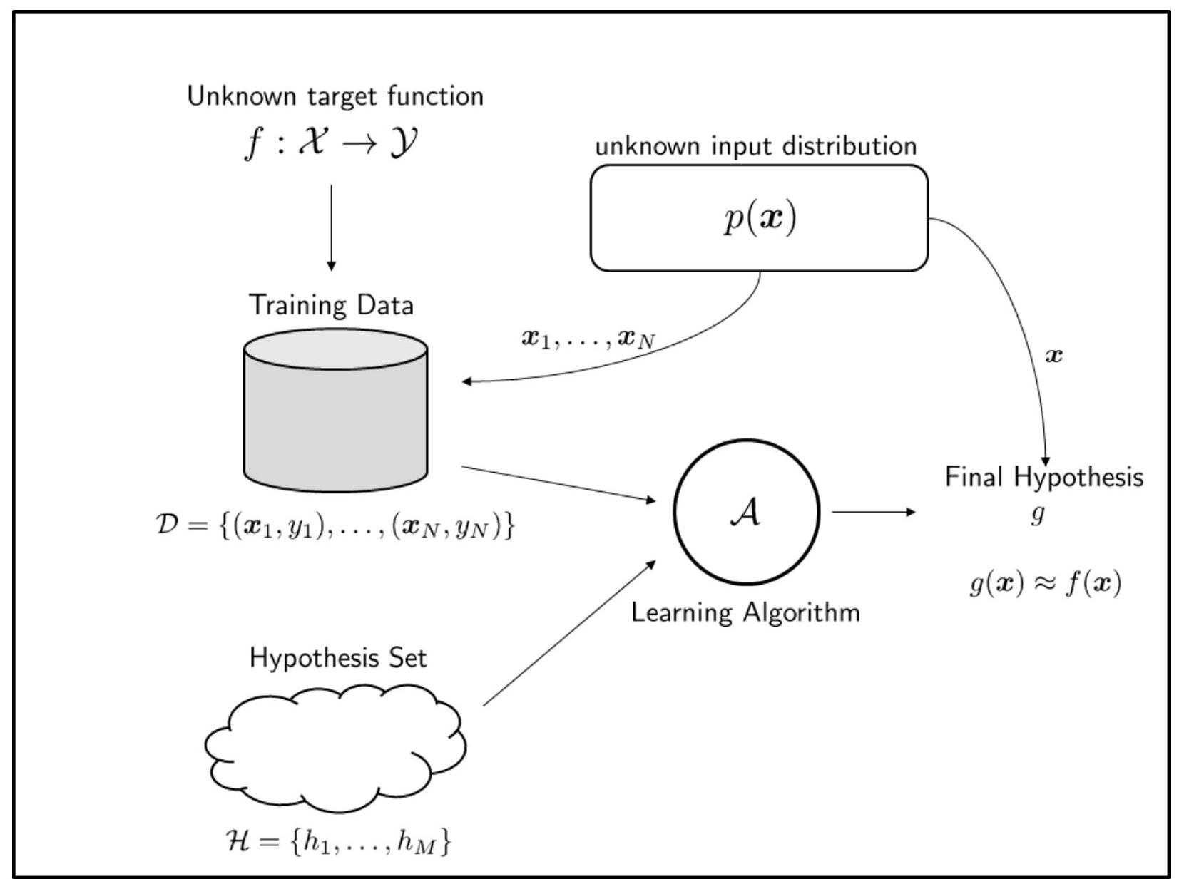
Fig. 16 All essential components of a machine learning model.

Is Learning Feasible?

The first question we ask is: Suppose we have a training set $\mathcal{S}$, can we learn the target function $f$ ? If the answer is YES, then we are all in business, because it means that we will be able to predict the data we have not seen. If the answer is NO, then machine learning is a lair and we should all go home, because it means that we can only memorize what we have seen but we will not be able to predict what we have not seen.

Interestingly, the answer to this question depends on how we define the training samples ${\mathbf{x}}^{(n)}$ ‘s. If ${\mathbf{x}}^{(n)}$ ‘s are deterministically defined, then the answer is NO because $\mathcal{S}$ can contain no information about the out-samples. Thus, there is no way to learn outside $\mathcal{S}$. If ${\mathbf{x}}^{(n)}$ ‘s are drawn from a probabilistic distribution, then the answer is YES because the distribution will tell us something about the out-samples. Let us look at these two situations one by one.

Learing Outside the Training Set $\mathcal{S}$ (Deterministic Case)

Let us look at the deterministic case. Consider a 3-dimensional input space $\mathcal{X}=\{0,1{\}}^3$. Each vector $\mathbf{x}\in \mathcal{X}$ is a binary vector containing three elements, e.g., $\mathbf{x}=[0,0,1{]}^T$ or $\mathbf{x}=[1,0,1{]}^T$. Since there are 3 elements and each element take a binary state, there are totally $2^3=8$ input vectors in $\mathcal{X}$.

How about the number of possible target functions $f$ can we have? Remember, a target function $f$ is a mapping which converts an input vector $\mathbf{x}$ to a label $y$. For simplicity let us assume that $f$ maps $\mathbf{x}$ to a binary output $y\in \{+1,-1\}$. Since there are 8 input vectors, we can think of $f$ as a 8-bit vector, e.g., $f=[-1,+1,-1,-1,-1,+1,+1,+1]$, where each entry represents the output. If we do the calculation, we can show that there are totally $2^8=256$ possible target functions.

Here is the learning problem. Can we learn $f$ from $\mathcal{S}$ ? To ensure that $f$ is unknown, we will not disclose what $f$ is. Instead, we assume that there is a training set $\mathcal{S}$ containing 6 training samples $\{{\mathbf{x}}^{(1)},\dots ,{\mathbf{x}}^{(6)}\}$. Corresponding to each ${\mathbf{x}}^{(n)}$ is the label $y^{(n)}$. The relationship between ${\mathbf{x}}^{(n)}$ and $y^{(n)}$ is shown in the table below. So our task is to pick a target function from the 256 possible choices.

Table 7 Truth Table for 6 samples

${\mathbf{x}}^{(n)}$	$y^{(n)}$
$[0,0,0]$	$\circ$
$[0,0,1]$	$\bullet$
$[0,1,0]$	$\bullet$
$[0,1,1]$	$\circ$
$[1,0,0]$	$\bullet$
$[1,0,1]$	$\circ$

Table 8 Function Table

${\mathbf{x}}^{(n)}$	$y^{(n)}$	$h_S$	$f_1$	$f_2$	$f_3$	$f_4$
$[0,0,0]$	$\circ$	$\circ$	$\circ$	$\circ$	$\circ$	$\circ$
$[0,0,1]$	$\bullet$	$\bullet$	$\bullet$	$\bullet$	$\bullet$	$\bullet$
$[0,1,0]$	$\bullet$	$\bullet$	$\bullet$	$\bullet$	$\bullet$	$\bullet$
$[0,1,1]$	$\circ$	$\circ$	$\circ$	$\circ$	$\circ$	$\circ$
$[1,0,0]$	$\bullet$	$\bullet$	$\bullet$	$\bullet$	$\bullet$	$\bullet$
$[1,0,1]$	$\circ$	$\circ$	$\circ$	$\circ$	$\circ$	$\circ$
$[1,1,0]$		$\circ /\bullet$	$\circ$	$\bullet$	$\circ$	$\bullet$
$[1,1,1]$		$\circ /\bullet$	$\circ$	$\circ$	$\bullet$	$\bullet$

Since we have seen 6 out of 8 input vectors in $\mathcal{S}$, there remains two input vectors we have not seen and need to predict. Thus, we can quickly reduce the number of possible target functions to $2^2=4$. Let us call these target functions $f_1,f_2,f_3$ and $f_4$. The boolean structure of these target functions are shown on the right hand side of the table above. Note that the first 6 entries of each $f_i$ is fixed because they are already observed in $\mathcal{S}$.

In the table above we write down the final hypothesis function $h_S$. The last two entries of $h_S$ is to be determined by the learning algorithm. If the learning algorithm decides $\circ$, then we will have both $\circ$. If the learning algorithm decides a $\circ$ followed by a $\bullet$, then we will have a $\circ$ followed by a $\bullet$. So the final hypothesis function $h_S$ can be one of the 4 possible choices, same number of choices of the target functions.

Since we assert that $f$ is unknown, by only observing the first 6 entries we will have 4 equally good hypothesis functions. They are equally good, because no matter which hypothesis function we choose, the last 2 entries will agree or disagree with the target depending on which one is the true target function. For example, on the left hand side of the table below, the true target function is $f_1$ and so our $h_S$ is correct. But if the true target function is $f_3$, e.g., the right hand side of the table, then our $h_S$ is wrong. We can repeat the experiment by choosing another $h_S$, and we can prove that not matter which $h_S$ we choose, we only have $25\mathrm{\%}$ chance of picking the correct one. This is the same as drawing a lottery from 4 numbers. The information we learned from the training set $\mathcal{S}$ does not allow us to infer anything outside $\mathcal{S}$.

Table 9 Function Table with $f_1$ as True Function

${\mathbf{x}}^{(n)}$	$y^{(n)}$	$h_S$	$f_1$	$f_2$	$f_3$	$f_4$
$[0,0,0]$	$\circ$	$\circ$	$\circ$	$\circ$	$\circ$	$\circ$
$[0,0,1]$	$\bullet$	$\bullet$	$\bullet$	$\bullet$	$\bullet$	$\bullet$
$[0,1,0]$	$\bullet$	$\bullet$	$\bullet$	$\bullet$	$\bullet$	$\bullet$
$[0,1,1]$	$\circ$	$\circ$	$\circ$	$\circ$	$\circ$	$\circ$
$[1,0,0]$	$\bullet$	$\bullet$	$\bullet$	$\bullet$	$\bullet$	$\bullet$
$[1,0,1]$	$\circ$	$\circ$	$\circ$	$\circ$	$\circ$	$\circ$
$[1,1,0]$		$\circ$	$\circ$	$\bullet$	$\circ$	$\bullet$
$[1,1,1]$		$\circ$	$\circ$	$\circ$	$\bullet$	$\bullet$

Table 10 Function Table with $f_3$ as True Function

${\mathbf{x}}^{(n)}$	$y^{(n)}$	$h_S$	$f_1$	$f_2$	$f_3$	$f_4$
$[0,0,0]$	$\circ$	$\circ$	$\circ$	$\circ$	$\circ$	$\circ$
$[0,0,1]$	$\bullet$	$\bullet$	$\bullet$	$\bullet$	$\bullet$	$\bullet$
$[0,1,0]$	$\bullet$	$\bullet$	$\bullet$	$\bullet$	$\bullet$	$\bullet$
$[0,1,1]$	$\circ$	$\circ$	$\circ$	$\circ$	$\circ$	$\circ$
$[1,0,0]$	$\bullet$	$\bullet$	$\bullet$	$\bullet$	$\bullet$	$\bullet$
$[1,0,1]$	$\circ$	$\circ$	$\circ$	$\circ$	$\circ$	$\circ$
$[1,1,0]$		$\circ$	$\circ$	$\bullet$	$\circ$	$\bullet$
$[1,1,1]$		$\circ$	$\circ$	$\circ$	$\bullet$	$\bullet$

The above analysis shows that learning is infeasible if we have a deterministic generator generating the training samples. The argument holds regardless which learning algorithm $\mathcal{A}$ we use, and what hypothesis set $\mathcal{H}$ we choose. Whether $\mathcal{H}$ contains the correct hypothesis function, and whether $\mathcal{A}$ can pick the correct hypothesis, there is no difference in terms of predicting outside $\mathcal{S}$. We can also extend the analysis from binary function to general learning problem. As long as $f$ remains unknown, it is impossible to predict outside $\mathcal{S}$.

Identically and Independently Distributed Random Variables

For the following section, we will discuss the case from a probabilistic perspective.

However, we will need to assume that the random variables are identically and independently distributed (i.i.d.). This means that the random variables are drawn from the same distribution and are independent of each other.

For formal definition, see Independent and Identically Distributed (IID).

This assumption is ubiquitous in machine learning. Not only does it simplify the analysis, it also solidifies many theories governing the framework underlying machine learning.

This assumption is a strong one and is not always true in practice. However, it is a reasonable one.

See extracted paragraph from Machine Learning Theory below:

This assumption is essential for us. We need it to start using the tools form probability theory to investigate our generalization probability, and it’s a very reasonable assumption because:

1. It’s more likely for a dataset used for inferring about an underlying probability distribution to be all sampled for that same distribution. If this is not the case, then the statistics we get from the dataset will be noisy and won’t correctly reflect the target underlying distribution.

2. It’s more likely that each sample in the dataset is chosen without considering any other sample that has been chosen before or will be chosen after. If that’s not the case and the samples are dependent, then the dataset will suffer from a bias towards a specific direction in the distribution, and hence will fail to reflect the underlying distribution correctly.

Learing Outside the Training Set $\mathcal{S}$ (Probabilistic Case)

The deterministic analysis gives us a pessimistic result. Now, let us look at a probabilistic analysis. On top of the training set $\mathcal{S}$, we pose an assumption. We assume that all $\mathbf{x}\in \mathcal{X}$ is drawn from a distribution ${\mathbb{P}}_{\mathcal{D}}(\mathbf{x})$. This includes all the in-samples ${\mathbf{x}}^{(n)}\in \mathcal{S}$ and the out-samples $\mathbf{x}\in \mathcal{X}$. At a first glance, putting a distributional assumption ${\mathbb{P}}_{\mathcal{D}}(\mathbf{x})$ does not seem any different from the deterministic case: We still have a training set $\mathcal{S}=\{{\mathbf{x}}^{(1)},\dots ,{\mathbf{x}}^{(N)}\}$, and $f$ is still unknown. How can we learn the unknown $f$ using just the training samples?

Suppose that we pick a hypothesis function $h$ from the hypothesis set $\mathcal{H}$. For every in-sample ${\mathbf{x}}^{(n)}$, we check whether the output returned by $h$ is the same as the output returned by $f$, i.e., $\{h\left({\mathbf{x}}^{(n)}\right)=f\left({\mathbf{x}}^{(n)}\right)\}$, for $n=1,\dots ,N$. If $\{h\left({\mathbf{x}}^{(n)}\right)=f\left({\mathbf{x}}^{(n)}\right)\}$, then we say that the in-sample ${\mathbf{x}}^{(n)}$ is correctly classified in the training. If $\{h\left({\mathbf{x}}^{(n)}\right)\ne f\left({\mathbf{x}}^{(n)}\right)\}$, then we say that ${\mathbf{x}}^{(n)}$ is incorrectly classified. Averaging over all the $N$ samples, we obtain a quantity called the in-sample error, or the training error. In our machine learning notations, the in-sample error is our Empirical Risk Minimization (ERM) function ${\mathcal{R}}_{\mathcal{S}}\left(h\right)$.

Definition 107 (Zero-One Loss)

The zero-one loss is defined as

(58)$$\mathcal{L}((\mathbf{x},y),h)=\mathbf{1}\{h\left(\mathbf{x}\right)\ne y\}$$

where $\mathbf{1}\{h\left(\mathbf{x}\right)\ne y\}$ is the indicator function that returns 1 if the condition is true, and 0 otherwise.

With this,

Definition 108 (In-Sample Error (Empirical Risk Minimization))

Consider a training set $\mathcal{S}=\{({\mathbf{x}}^{(1)},y^{(1)}),({\mathbf{x}}^{(2)},y^{(2)}),\dots ,({\mathbf{x}}^{(N)},y^{(N)})\}\stackrel{\text{iid}}{\sim }{\mathbb{P}}_{\mathcal{D}}$, and a target function $f$. The in-sample error (or the training error) of a hypothesis function $h\in \mathcal{H}$ is the empirical average of the zero-one loss $\mathcal{L}((\mathbf{x},y),h):=\{h\left({\mathbf{x}}^{(n)}\right)\ne f\left({\mathbf{x}}^{(n)}\right)\}$ :

(59)$$\begin{array}{r}\begin{array}{rl}{\hat{\mathcal{R}}}_{\mathcal{S}}\{\mathcal{L}((\mathbf{x},y),h)\}:& =\frac{1}{N}\sum _{n=1}^N\mathcal{L}(({\mathbf{x}}^{(n)},y^{(n)}),h)\\ & =\frac{1}{N}\sum _{n=1}^N\mathbf{1}\{h\left({\mathbf{x}}^{(n)}\right)\ne f\left({\mathbf{x}}^{(n)}\right)\}\\ & ={\mathbb{E}}_{\mathcal{S}}\left[\mathcal{L}((\mathbf{x},y),h)\right]\end{array}\end{array}$$

Training error is the amount of error we have during the training process. A good learning algorithm $\mathcal{A}$ should pick a hypothesis $h$ that gives low training error. Training error is sometimes called the cost (empirical risk) function (or the loss function) when we post the learning problem as an optimization. Thus, picking a good hypothesis is equivalent to minimizing the training error.

How about the out-samples? Since we assume that $\mathbf{x}$ is drawn from a distribution ${\mathbb{P}}_{\mathcal{D}}(\mathbf{x})$, we can define the out-sample error as the probability that $\{h(\mathbf{x})\ne f(\mathbf{x})\}$, for all $\mathbf{x}\sim {\mathbb{P}}_{\mathcal{D}}(\mathbf{x})$.

Definition 109 (Out-Sample Error (Generalization Error))

Consider an input space $\mathcal{X}$ containing elements $\mathbf{x}$ drawn from a distribution ${\mathbb{P}}_{\mathcal{D}}$, and a target function $f$. The out-sample error (or the true risk/testing error) of a hypothesis function $h\in \mathcal{H}$ is

$$\begin{array}{r}\begin{array}{rl}{\mathcal{R}}_{\mathcal{D}}\{\mathcal{L}((\mathbf{x},y),h)\}:& =\mathbb{P}\left[\{h\left(\mathbf{x}\right)\ne f\left(\mathbf{x}\right)\}\right]\\ & ={\mathbb{E}}_{\mathcal{D}}[\mathcal{L}((\mathbf{x},y),h)]\\ & ={\mathbb{E}}_{\mathcal{D}}\left[\mathbf{1}\{h\left(\mathbf{x}\right)\ne f\left(\mathbf{x}\right)\}\right]\end{array}\end{array}$$

where $\mathbb{P}[\cdot ]$ measures the probability of the statement based on the distribution ${\mathbb{P}}_{\mathcal{D}}(\mathbf{x})$.

How did we derive from a probability of classifying one sample wrongly to the expectation over the loss function?

Since $\mathbf{1}$ is a binary function, the out-sample error is the expected value of a sample being misclassified over the entire distribution:

$$\begin{array}{r}\begin{array}{rl}{\mathcal{R}}_{\mathcal{D}}\{\mathcal{L}((\mathbf{x},y),h)\}=& \mathbb{P}[h(\mathbf{x})\ne f(\mathbf{x})]\\ =& \underset{=1}{\underbrace{{\mathbf{1}}_{h\left({\mathbf{x}}^{(n)}\right)\ne f\left({\mathbf{x}}^{(n)}\right)}}}\mathbb{P}\{h\left({\mathbf{x}}^{(n)}\right)\ne f\left({\mathbf{x}}^{(n)}\right)\}\\ & +\underset{=0}{\underbrace{{\mathbf{1}}_{h\left({\mathbf{x}}^{(n)}\right)=f\left({\mathbf{x}}^{(n)}\right)}}}(1-\mathbb{P}\{h\left({\mathbf{x}}^{(n)}\right)\ne f\left({\mathbf{x}}^{(n)}\right)\})\\ =& {\mathbb{E}}_{\mathcal{D}}\left\{{\mathbf{1}}_{h\left({\mathbf{x}}^{(n)}\right)\ne f\left({\mathbf{x}}^{(n)}\right)}\right\}.\end{array}\end{array}$$

Therefore, the relationship between the in-sample error ${\hat{\mathcal{R}}}_{\mathcal{S}}\{\mathcal{L}((\mathbf{x},y),h)\}$ and out-sample error ${\mathcal{R}}_{\mathcal{D}}\{\mathcal{L}((\mathbf{x},y),h)\}$ is equivalent to the relationship between the empirical average and the population mean of a random variable, where the random variable is the loss function $\mathcal{L}$.

Fig. 17 shows how an in-sample error is computed.

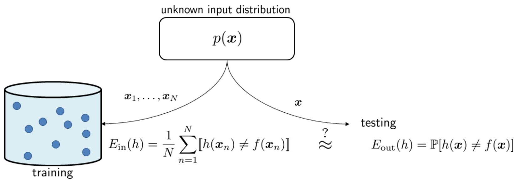
Fig. 17 ${\hat{\mathcal{R}}}_{\mathcal{S}}$ is evaluated using the training data, whereas ${\mathcal{R}}_{\mathcal{D}}$ is evaluated using the testing sample. Here the author uses ${\mathbb{E}}_{\text{in}}$ and ${\mathbb{E}}_{\text{out}}$ to denote the in-sample and out-sample error, respectively.

To this end, we recap of what we have:

We have a hypothesis space $\mathcal{H}$ of functions that we can use to approximate the underlying distribution. We have a loss function $\mathcal{L}$ that we can use to measure the quality of our approximation. We have a learning algorithm that can be used to find the best function in $\mathcal{H}$ that approximates the underlying distribution $\mathcal{D}$. We have a test dataset ${\mathcal{S}}_{\text{test}}$ sampled $\mathbf{\text{i.i.d.}}$ from the underlying and unknown distribution $\mathcal{D}$.

We want to know the probability that our learning algorithm will find a function in $\mathcal{H}$ that approximates the underlying distribution $\mathcal{D}$ well enough to generalize well to the test dataset ${\mathcal{S}}_{\text{test}}$.

In other words, the learning problem at hand is to find a hypothesis $h\in \mathcal{H}$ that minimizes the expected risk $\hat{\mathcal{R}}$ over the training samples $\mathcal{S}$ which is generated by the underlying unknown true distribution $\mathcal{D}$ such that the generalization risk/error $\mathcal{R}\le \hat{\mathcal{R}}+ϵ$ with high probability.

How can we do that? Let’s start with the Law of Large Numbers.

Remark 28 (Notation)

It should be clear from context that $\mathcal{R}$ is the generalization error of the hypothesis $h$ over the entire distribution $\mathcal{D}$. In other words, this is the expected error based on the entire distribution $\mathcal{D}$.

On the other hand, $\hat{\mathcal{R}}$ is the empirical risk of the hypothesis $h$ over the training samples $\mathcal{S}$.

The Generalization Gap

Definition 110 (Generalization Gap)

Given a sample set $\mathcal{S}={\left\{({\mathbf{x}}^{(n)},y^{(n)})\right\}}_{n=1}^N$ drawn $\mathbf{\text{i.i.d.}}$ from the distribution $\mathcal{D}$, a hypothesis $h_S\in \mathcal{H}$ learnt by the algorithm $\mathcal{A}$ on $\mathcal{S}$, and a specific definition of loss function $\mathcal{L}$ (i.e. zero-one loss), the generalization gap is defined as:

$$\begin{array}{r}{ϵ}_{gen}(h_S)=|{\mathcal{R}}_{\mathcal{D}}\{\mathcal{L}((\mathbf{x},y),h_S)\}-{\hat{\mathcal{R}}}_{\mathcal{S}}\{\mathcal{L}((\mathbf{x},y),h_S)\}|.\end{array}$$

The Law of Large Numbers

Recall that in the section Empirical Risk Minimization approximates True Risk Minimization of the chapter on ERM, we mentioned that the the Empirical Risk approximates the True Risk as the number of samples $N$ grows. This is the Law of Large Numbers that was mentioned in an earlier chapter.

We restate the Weak Law of Large Numbers from Theorem 55 below again, but with notation more aligned to our notations in machine learning notations chapter. In particular, we use $\mathcal{L}$ suggesting that the random variable is the loss value of $\mathcal{L}(\cdot )$. In other words, ${\mathcal{L}}^{(n)}$ is treated as realizations of the random variable $\mathcal{L}$ on the $n$-th sample.

Theorem 60 (Weak Law of Large Numbers)

Let ${\mathcal{L}}^{(1)},\dots ,{\mathcal{L}}^{(N)}$ be $\mathbf{\text{i.i.d.}}$ random variables with common mean $\mu$ and variance ${\sigma }^2$. Each $\mathcal{L}$ is distributed by the same probability distribution $\mathbb{P}$ ($\mathcal{D}$).

Let $\overline{\mathcal{L}}$ be the sample average defined in (43) and $\mathbb{E}[{\mathcal{L}}^2]<\mathrm{\infty }$.

Then, for any $ϵ>0$, we have

(60)$$\underset{N\to \mathrm{\infty }}{lim}\mathbb{P}[|\underset{\mathcal{L}\sim P}{\mathbb{E}}[\mathcal{L}]-\frac{1}{N}\sum _{n=1}^N{\mathbf{x}}^{(n)}|>ϵ]:=\underset{N\to \mathrm{\infty }}{lim}\mathbb{P}[|\mu -{\overline{\mathcal{L}}}^{(N)}|>ϵ]=0$$

This means that

(61)$$\overline{\mathcal{L}}\stackrel{p}{\to }\underset{\mathcal{L}\sim P}{\mathbb{E}}[\mathcal{L}]\text{as }N\to \mathrm{\infty }$$

In other words, as sample size $N$ grows, the probability that the sample average $\overline{\mathcal{L}}$ differs from the population mean $\mu$ by more than $ϵ$ approaches zero. Note this is not saying that the probability of the difference between the sample average and the population mean is more than epsilon is zero, the expression is the probability that the difference is more than epsilon! So in laymen terms, as $N$ grows, then it is guaranteed that the difference between the sample average and the population mean is no more than $ϵ$. This seems strong since $ϵ$ can be arbitrarily small, but it is still a probability bound.

Then recall that the True Risk Function is defined as:

$${\mathcal{R}}_{\mathcal{D}}\{\mathcal{L}((\mathbf{x},y),h)\}:={\mathbb{E}}_{\mathcal{D}}[\mathcal{L}((\mathbf{x},y),h)]$$

and the Empirical Risk Function is defined as:

$${\hat{\mathcal{R}}}_{\mathcal{S}}\{\mathcal{L}((\mathbf{x},y),h)\}:=\frac{1}{N}\sum _{n=1}^N\mathcal{L}(({\mathbf{x}}^{(n)},y^{(n)}),h)$$

Furthermore, since $\mathcal{L}$ is defined to be a random variable representing the loss/error of a single sample, then we can rewrite the True Risk Function as:

$${\mathcal{R}}_{\mathcal{D}}\{\mathcal{L}((\mathbf{x},y),h)\}:={\mathbb{E}}_{\mathcal{D}}\left[\mathcal{L}((\mathbf{x},y),h)\right]$$

which means that the True Risk Function is the expected loss/error of all possible samples. This is because we treat $\mathcal{L}$ as a random variable and we take the expected value of it.

Remark 29 (Random Variable is a Function)

The notation might seem overloaded and abused, but since random variable in itself is a function, and $\mathcal{L}(\cdot )$ is also a function mapping states $(\mathbf{x},y)$ to a real number, then we can treat $\mathcal{L}$ as a random variable representing the loss/error of a single sample.

Now, define ${\mathcal{L}}^{(n)}$ to be the loss/error of the $n$-th sample in the train dataset $\mathcal{S}$. Then we can rewrite the Empirical Risk Function as:

$${\hat{\mathcal{R}}}_{\mathcal{S}}\{\mathcal{L}((\mathbf{x},y),h)\}:=\frac{1}{N}\sum _{n=1}^N{\mathcal{L}}^{(n)}$$

which means that the Empirical Risk Function is the average loss/error of all training samples.

Notice that they both have exactly the same form as the Weak Law of Large Numbers, so we can apply the Weak Law of Large Numbers to the True Risk Function and the Empirical Risk Function. This natural application of the Weak Law of Large Numbers allows us to answer the following question (also in (57)):

Remark 30 (Summary)

Given a dataset $\mathcal{S}={\left\{({\mathbf{x}}^{(n)},y^{(n)})\right\}}_{n=1}^N$, and a fixed and single hypothesis $h$, the Weak Law of Large Numbers tells us that as the number of samples in your training set increases from $N$ to $\mathrm{\infty }$, the Empirical Risk Function will converge to the True Risk Function.

(62)$$\underset{N\to \mathrm{\infty }}{lim}\mathbb{P}[|{\mathcal{R}}_{\mathcal{D}}(h)-{\hat{\mathcal{R}}}_{\mathcal{S}}(h)|>ϵ]=0$$

where the notation of $\mathcal{R}$ and $\hat{\mathcal{R}}$ are simplified to only contain $h$ for readability.

Well, this is something. At least we know that if we can bump up the number of samples in our training set to $\mathrm{\infty }$, then we can guarantee that the Empirical Risk Function will be close to the True Risk Function. But this is not really very useful, because we can’t really get $\mathrm{\infty }$ samples in practice.

Can we do better by finding an upper bound on the right hand side of (62)? This bound has to be a function of the number of samples $N$ so we at least know how many samples we need to get a good approximation of the True Risk Function, or even if we cannot get more samples, then what is the theoretical maximum error we can expect from the Empirical Risk Function?

Hoeffding’s Inequality

Earlier, we also saw the discussion of this inequality in a previous chapter. This inequality will help us answer the question above.

We restate the Hoeffding’s Inequality here, but in machine learning context:

Theorem 61 (Hoeffding’s Inequality)

Consider a dataset $\mathcal{S}={\left\{({\mathbf{x}}^{(n)},y^{(n)})\right\}}_{n=1}^N$ drawn i.i.d. from an unknown distribution $\mathcal{D}$. Let the hypothesis set $\mathcal{H}=\{h_1,\dots ,h_K\}$ be a finite set of hypotheses. Then, suppose we fix a hypothesis $h$ in $\mathcal{H}$ (for any $h\in \mathcal{H}$) before we look at the dataset $\mathcal{S}$, which means we have not learnt $h_S$ yet.

Furthermore, let $\mathcal{L}((\mathbf{x},y),h)$ be the loss/error of a single sample $(\mathbf{x},y)$ with respect to the hypothesis $h$ such that $0\le \mathcal{L}((\mathbf{x},y),h)\le 1$ and $\mathbb{E}[\mathcal{L}((\mathbf{x},y),h)]$ be the expected loss/error over the entire distribution $\mathcal{D}$.

We can then define a sequence of random variables ${\left\{{\mathcal{L}}^{(n)}\right\}}_{n=1}^N$ such that ${\mathcal{L}}^{(n)}$ is the loss/error of the $n$-th sample in the dataset $\mathcal{S}$.

Then for any $ϵ>0$, we have the following bound:

$$\begin{array}{r}\begin{array}{rl}\mathbb{P}[|\mathbb{E}[\mathcal{L}((\mathbf{x},y),h)]-\frac{1}{N}\sum _{n=1}^N{\mathcal{L}}^{(n)}(({\mathbf{x}}^{(n)},y^{(n)}),h)|>ϵ]& =\mathbb{P}[|{\mathcal{R}}_{\mathcal{D}}(h)-{\hat{\mathcal{R}}}_{\mathcal{S}}(h)|>ϵ]\\ & \le 2e^{-2{ϵ}^{2}N}\end{array}\end{array}$$

where $N$ is the number of samples in the dataset $\mathcal{S}$, and $\mathcal{R}$ and $\hat{\mathcal{R}}$ are the True Risk Function and the Empirical Risk Function respectively.

Remark 31 (Things to Note (Important))

1. Note that both $\mathcal{L}((\mathbf{x},y),h)$ and the samples $({\mathbf{x}}^{(n)},y^{(n)})$ are drawn from the same distribution $\mathcal{D}$.

2. Important: Note carefully this $h$ is even picked even before the dataset $\mathcal{S}$ is generated from $\mathcal{D}$. This is not a trivial concept and requires quite some justification. See Why must h be fixed and defined before generating the dataset \mathcal{S}?.

3. The random variable must be bounded between $0$ and $1$, so your loss function must be bounded between $0$ and $1$. This is simple to do usually since you usually apply sigmoid/softmax to your output to get a probability between $0$ and $1$ to feed into your loss function.

As the number of training samples $N$ grows, the in-sample error ${\hat{\mathcal{R}}}_{\mathcal{S}}(h)$ (which is the training error) converges exponentially to the out-sample error ${\mathcal{R}}_{\mathcal{D}}(h)$ (which is the testing error). The in-sample error ${\hat{\mathcal{R}}}_{\mathcal{S}}(h)$ is something we can compute numerically using the training set. The out-sample error is an unknown quantity because we do not know the target function $f$. Hoeffding inequality says even though we do not know ${\hat{\mathcal{R}}}_{\mathcal{S}}(h)$, for large enough $N$ the in-sample error ${\hat{\mathcal{R}}}_{\mathcal{S}}(h)$ will be sufficiently close to ${\mathcal{R}}_{\mathcal{D}}(h)$. Therefore, we will be able to tell how good the hypothesis function is without accessing the unknown target function.

Comparing Hoeffding’s Inequality with the Chebyshev’s Inequality

Let us take a quick comparison between the Hoeffding inequality and the Chebyshev inequality. Chebyshev inequality states that

$$\mathbb{P}[|\mathbb{E}[\mathcal{L}((\mathbf{x},y),h)]-\frac{1}{N}\sum _{n=1}^N{\mathcal{L}}^{(n)}|>ϵ]\le \frac{{\sigma }^2}{{ϵ}^{2}N}.$$

where ${\sigma }^2$ is the variance of the loss/error $\mathcal{L}((\mathbf{x},y),h)$.

If we let $2e^{-2{ϵ}^{2}N}\le \delta$ for some $\delta$ in Hoeffding inequality, and $\frac{{\sigma }^2}{{ϵ}^{2}N}$ for some $\delta$ in Chebyshev inequality, we can easily see that the two inequalities imply

$$N\ge -\frac{1}{2{ϵ}^2}\log \frac{\delta }{2},\text{ and }N\ge \frac{{\sigma }^2}{{ϵ}^2\delta }.$$

For simplicity let us assume that $\sigma =1,ϵ=0.1$ and $\delta =0.01$. Then the above calculation will give $N\ge 265$ for Hoeffding whereas $N\ge 10000$ for Chebyshev. That means, Hoeffding inequality has a much lower prediction of how many samples we need to achieve an error of $\delta \le 0.01$.

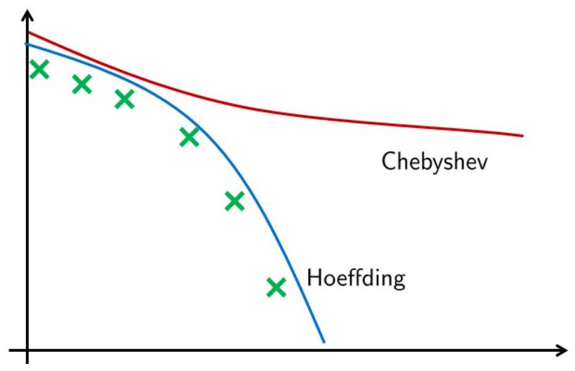
Fig. 18 Comparing Hoeffding inequality and Chebyshev inequality to predict the actual probability bound.

We see that Chebyshev is a more conservative bound than Hoeffding, and is less strong than Hoeffding since Hoeffding does not need to know anything about the random variable $\mathcal{L}((\mathbf{x},y),h)$ on the right hand side of the inequality.

Example: Hoeffding’s Inequality in Classification

Notation may be slightly different from the rest of the section.

Following exampled adapted from STAT425.

A powerful feature of the Hoeffding’s inequality is that it holds regardless of the classifier. Namely, even if we are considering many different types of classifiers, some are decision trees, some are kNN, some are logistic regression, they all satisfy equation above.

What this means is this inequality holds for any classifier $h$ and any loss function $\mathcal{L}$.

So even if your loss function is not $0-1$ loss, you can still use the Hoeffding’s inequality. Say cross-entropy loss, then you just need to know that the difference between the expected loss of the classifier and the empirical loss of the classifier is bounded by the right hand side of the inequality.

PAC Framework

The probabilistic analysis is called a probably approximately correct (PAC) framework. The word $\mathrm{P}-\mathrm{A}-\mathrm{C}$ comes from three principles of the Hoeffding inequality:

• Probably: We use the probability $\mathbb{P}[|{\mathcal{R}}_{\mathcal{D}}\{\mathcal{L}((\mathbf{x},y),h)\}-{\hat{\mathcal{R}}}_{\mathcal{S}}\{\mathcal{L}((\mathbf{x},y),h)\}|>ϵ]\le 2e^{-2{ϵ}^{2}N}$ as a measure to quantify the error.

• Approximately: The in-sample error is an approximation of the out-sample error, as given by $\mathbb{P}\left[|{\mathcal{R}}_{\mathcal{D}}\{\mathcal{L}((\mathbf{x},y),h)\}-{\hat{\mathcal{R}}}_{\mathcal{S}}\{\mathcal{L}((\mathbf{x},y),h)\}|>ϵ\right]\le 2e^{-2{ϵ}^{2}N}$. The approximation error is controlled by $ϵ$.

• Correct: The error is bounded by the right hand side of the Hoeffding inequality: $\mathbb{P}[|{\mathcal{R}}_{\mathcal{D}}\{\mathcal{L}((\mathbf{x},y),h)\}-{\hat{\mathcal{R}}}_{\mathcal{S}}\{\mathcal{L}((\mathbf{x},y),h)\}|>ϵ]\le 2e^{-2{ϵ}^{2}N}$. The accuracy is controlled by $N$ for a fixed $ϵ$.

Hoeffding Inequality is Invalid for $h_S$ learnt from $\mathcal{S}$

Now, there is one last problem we need to resolve. The above Hoeffding inequality holds for a fixed hypothesis function $h$. This means that $h$ is already chosen before we generate the dataset. If we allow $h$ to change after we have generated the dataset, then the Hoeffding inequality is no longer valid. What do we mean by after generating the dataset? In any learning scenario, we are given a training dataset $\mathcal{S}$. Based on this dataset, we have to choose a hypothesis function $h_S$ from the hypothesis set $\mathcal{H}$. The hypothesis $h_S$ we choose depends on what samples are inside $\mathcal{S}$ and which learning algorithm $\mathcal{A}$ we use. So $h_S$ changes after the dataset is generated.

Now this is a non-trivial problem, and to fully understand this requires close scrutiny. Recall in Remark 31’s point 2, we said that $h$ is fixed prior to generating the dataset $\mathcal{S}$ and using $\mathcal{A}$ to learn $h_S$ from $\mathcal{S}$.

Here are some links that explains the issue in details on where exactly the problem lies. All in all, one just needs to know that the assumption of $\mathbf{\text{i.i.d.}}$ is broken in Hoeffding’s Inequality if you allow $h$ to change to $h_S$ after learning from $\mathcal{S}$.

• 1. Why is Hoeffding’s inequality invalid if we use $h_S$ instead of $h$?

• 2. Why is Hoeffding’s inequality invalid if we use $h_S$ instead of $h$?

• 3. Why is Hoeffding’s inequality invalid if we use $h_S$ instead of $h$?

---

This has serious implications! The logic that follows is that before learning, for any fixed $h$, we can bound the error by the Hoeffding’s Inequality. But now, there is no guarantee that $|{\mathcal{R}}_{\mathcal{D}}(h_S)-{\hat{\mathcal{R}}}_{\mathcal{S}}(h_S)|>ϵ$ (the “bad event”) is less than $\delta$ (the “bad event probability”). It could be less, it could be more, no one knows, but we do know that $h_S\in \mathcal{H}$.

Let’s see how we can make use of this property to bound the error for the entire hypothesis set $\mathcal{H}$ instead of just a single hypothesis $h$.

Union Bound

Suppose that $\mathcal{H}$ contains $M$ hypothesis functions $h_1,\dots ,h_M$. The final hypothesis $h_S$ that your learning algorithm $\mathcal{A}$ picked is one of these potential hypotheses. To have $|{\mathcal{R}}_{\mathcal{D}}(h_S)-{\hat{\mathcal{R}}}_{\mathcal{S}}(h_S)|>ϵ$, we need to ensure that at least one of the $M$ potential hypotheses can satisfy the inequality.

Remark 32 (Bounding the Entire Hypothesis Set)

This part helps visualize why you need to use union bound to bound all hypotheses in $\mathcal{H}$.

This is best read together with the example in Wikipedia.

First, we must establish that for the $h_S$ learnt by $\mathcal{A}$ on the dataset $\mathcal{S}$, the generalization gap $|{\mathcal{R}}_{\mathcal{D}}(h_S)-{\hat{\mathcal{R}}}_{\mathcal{S}}(h_S)|$ is no longer bounded by the Hoeffding Inequality. We turn our attention to bounding the entire hypothesis set $\mathcal{H}$ instead of just a single hypothesis $h$.

Second, let us define the bad event $\mathcal{B}$ to be:

$$\mathcal{B}=\{|{\mathcal{R}}_{\mathcal{D}}(h_S)-{\hat{\mathcal{R}}}_{\mathcal{S}}(h_S)|>ϵ\}$$

which is the event that the error is greater than $ϵ$.

Then it follows that ${\mathcal{B}}_m$ is the bad event for the $m$th hypothesis $h_m$ in $\mathcal{H}$:

$${\mathcal{B}}_m=\{|{\mathcal{R}}_{\mathcal{D}}(h_m)-{\hat{\mathcal{R}}}_{\mathcal{S}}(h_m)|>ϵ\}$$

We define the good event ${\mathcal{B}}^{\mathrm{c}}$ to be the good event, the complement of the bad event to be:

$${\mathcal{B}}^{\mathrm{c}}=\{|{\mathcal{R}}_{\mathcal{D}}(h_S)-{\hat{\mathcal{R}}}_{\mathcal{S}}(h_S)|\le ϵ\}$$

which is the event that the error is less than or equal to $ϵ$.

Third, we want to show that $\mathrm{\forall }{h}_m\in \mathcal{H}$, the probability of all $h_1,h_2\dots ,h_M$ is bounded below by a value of say, $\varphi$.

In other words, denote the event $\mathcal{C}$ as the event where all $h_1,h_2\dots ,h_M$ are “good” (none of them are “bad”). The event $\mathcal{C}$ can be defined as:

$$\mathcal{C}={{\mathcal{B}}_{\mathcal{1}}}^{\mathrm{c}}\cap {{\mathcal{B}}_{\mathcal{2}}}^{\mathrm{c}}\cap \dots \cap {{\mathcal{B}}_{\mathcal{M}}}^{\mathrm{c}}$$

which is the event that all $h_1,h_2\dots ,h_M$ are “good”. Now, we seek to find the probability of $\mathcal{C}$ to be greater than or equal to $\varphi$.

$$\begin{array}{r}\begin{array}{rl}\mathbb{P}\left(\mathcal{C}\right)& >\varphi \end{array}\end{array}$$

For example, if $\varphi =0.95$, this means that we can be 95% confident that all $h_1,h_2\dots ,h_M$ are “good” (i.e. all $h_1,h_2,\dots ,h_M$ give a generalization error less than or equal to $ϵ$).

However, to make use of Union Bound (Boole’s Inequality), we need to express the $h_1,h_2,\dots ,h_M$ as a sequence of logical or events. Let’s try to rephrase the event $\mathcal{C}$ as a sequence of logical or events.

Fourth, let ${\mathcal{C}}^{\mathrm{c}}$ be the complement of the event $\mathcal{C}$:

$$\begin{array}{r}\begin{array}{rl}{\mathcal{C}}^{\mathrm{c}}& =\mathrm{\exists }{h}_m\in \mathcal{H}\text{s.t.}{h}_m\text{ is a bad}\\ & ={\mathcal{B}}_{\mathcal{1}}\cup {\mathcal{B}}_{\mathcal{2}}\cup \dots \cup {\mathcal{B}}_{\mathcal{M}}\\ & =h_1\text{ gives a bad error}\cup h_2\text{ gives a bad error}\cup \dots \cup h_M\text{ gives a bad error}\end{array}\end{array}$$

Then, finding $\mathbb{P}(\mathcal{C})>\varphi$ is equivalent to finding the following:

$$\begin{array}{r}\begin{array}{rlr}& \mathbb{P}\left(\mathcal{C}\right)& >\varphi \\ ⟺& 1-\mathbb{P}\left({\mathcal{C}}^{\mathrm{c}}\right)& >\varphi \\ ⟺& \mathbb{P}\left({\mathcal{C}}^{\mathrm{c}}\right)& \le 1-\varphi \end{array}\end{array}$$

where we invoked that $\mathcal{C}+{\mathcal{C}}^{\mathrm{c}}=1$. Now, we have turned the problem of finding $\mathbb{P}(\mathcal{C})>\varphi$ into finding the probability of ${\mathcal{C}}^{\mathrm{c}}$ to be less than or equal to $1-\varphi$ (from lower bound to upper bound).

Fifth, so now we can instead find the equivalent of the Hoeffding Inequality for the event ${\mathcal{C}}^{\mathrm{c}}$:

$$\begin{array}{r}\begin{array}{rl}\mathbb{P}\left({\mathcal{C}}^{\mathrm{c}}\right)& =\mathbb{P}({\mathcal{B}}_{\mathcal{1}}\cup {\mathcal{B}}_{\mathcal{2}}\cup \dots \cup {\mathcal{B}}_{\mathcal{M}})\\ & \le \mathbb{P}\left({\mathcal{B}}_{\mathcal{1}}\right)+\mathbb{P}\left({\mathcal{B}}_{\mathcal{2}}\right)+\dots +\mathbb{P}\left({\mathcal{B}}_{\mathcal{M}}\right)\end{array}\end{array}$$

where we invoked the Union Bound (Boole’s Inequality).

Last, in order for the entire hypothesis space to have a generalization gap bigger than $ϵ$, at least one of its hypothesis: $h_1$ or $h_2$ or $h_3$ or … etc should have. This can be expressed formally by stating that:

$$\mathbb{P}[\underset{h\in \mathcal{H}}{sup}|\mathcal{R}(h)-\hat{\mathcal{R}}(h)|>ϵ]=\mathbb{P}[\bigcup _{h\in \mathcal{H}}|\mathcal{R}(h)-\hat{\mathcal{R}}(h)|>ϵ]$$

Where $\bigcup$ denotes the union of the events, which also corresponds to the logical OR operator. Using the union bound inequality, we get:

(63)$$\begin{array}{r}\begin{array}{rl}\mathbb{P}\{|{\hat{\mathcal{R}}}_{\mathcal{D}}(h_S)-{\mathcal{R}}_{\mathcal{S}}(h_S)|>ϵ\}& \stackrel{(a)}{\le }\mathbb{P}[\underset{h\in \mathcal{H}}{sup}|\mathcal{R}(h)-\hat{\mathcal{R}}(h)|>ϵ]\\ & =\mathbb{P}[\bigcup _{h\in \mathcal{H}}|\mathcal{R}(h)-\hat{\mathcal{R}}(h)|>ϵ]\\ & \stackrel{(b)}{\le }\sum _{m=1}^M\mathbb{P}\{|{\hat{\mathcal{R}}}_{\mathcal{D}}\left(h_m\right)-{\mathcal{R}}_{\mathcal{S}}\left(h_m\right)|>ϵ\}\\ & =\sum _{m=1}^{M}2e^{-2{ϵ}^{2}N}\\ & =\left|\mathcal{H}\right|2e^{-2{ϵ}^{2}N}\text{. }\end{array}\end{array}$$

where $(a)$ holds because $\mathbb{P}[A]\le \mathbb{P}[B]$ if $A\Rightarrow B$, and $(b)$ is the Union bound which says $\mathbb{P}[A$ or $B]\le \mathbb{P}[A]+\mathbb{P}[B]$.

Therefore, if we bound each $h_m$ using the Hoeffding inequality

$$\mathbb{P}\{|{\hat{\mathcal{R}}}_{\mathcal{S}}\left(h_m\right)-{\mathcal{R}}_{\mathcal{D}}\left(h_m\right)|>ϵ\}\le 2e^{-2{ϵ}^{2}N}$$

then the overall bound on $h_S$ is the sum of the $M$ terms.

To see why $(a)$ holds, consider the following:

$$\begin{array}{r}\begin{array}{rl}|{\hat{\mathcal{R}}}_{\mathcal{D}}(g)-{\mathcal{R}}_{\mathcal{S}}(g)|>ϵ& ⟹\{|{\hat{\mathcal{R}}}_{\mathcal{D}}\left(h_1\right)-{\mathcal{R}}_{\mathcal{S}}\left(h_1\right)|>ϵ\text{ or }|{\hat{\mathcal{R}}}_{\mathcal{D}}\left(h_2\right)-{\mathcal{R}}_{\mathcal{S}}\left(h_2\right)|>ϵ\text{ or }\dots \text{ or }|{\hat{\mathcal{R}}}_{\mathcal{D}}\left(h_M\right)-{\mathcal{R}}_{\mathcal{S}}\left(h_M\right)|>ϵ\}\end{array}\end{array}$$

The LHS is event $A$ for example, the RHS is event $B$, then since we have $A\Rightarrow B$, we have $\mathbb{P}[A]\le \mathbb{P}[B]$.

Thus, we found a bound for the whole hypothesis set $\mathcal{H}$. Thus our $1-\varphi$ is actually $\left|\mathcal{H}\right|2e^{-2{ϵ}^{2}N}$.

Click to show

The below content was what I initially wrote, but the argument is hand-wavy, so I tried to lay out the argument more formally above. Still quite unsure if the reasoning is correct, but at least should be along those lines.

If one has $M$ hypotheses $h_1,\dots ,h_M$ in $\mathcal{H}$, then what is the probability that all $M$ hypotheses satisfy the inequality $|{\mathcal{R}}_{\mathcal{D}}(h_S)-{\hat{\mathcal{R}}}_{\mathcal{S}}(h_S)|\le ϵ$? So if our probability found is $95\mathrm{\%}$, this means that we can be 95% confident that all $M$ hypotheses satisfy the inequality. This is setting $\delta =0.05$.

$$\begin{array}{r}\mathbb{P}(|{\mathcal{R}}_{\mathcal{D}}(h_S)-{\hat{\mathcal{R}}}_{\mathcal{S}}(h_S)|\le ϵ)\ge 1-\delta \end{array}$$

If we can find this probability, then this just means that whichever $h_S$ we learnt by $\mathcal{A}$ on $\mathcal{S}$, will have an error less than or equal to $ϵ$ with probability $95\mathrm{\%}$ (similar to confidence interval).

We are stating the problem by asking the event “all $M$ hypotheses are good”, now we can find the complement of “all $M$ hypotheses are good” to be “at least one $h_m$ is bad” so that we can use the union bound easier.

Now, if we go the route of finding complement, then this objective is stated as:

If one has $M$ hypotheses $h_1,\dots ,h_M$ in $\mathcal{H}$, then what is the probability that at least (there exists) at least one $h_m$ such that $|{\mathcal{R}}_{\mathcal{D}}(h_m)-{\hat{\mathcal{R}}}_{\mathcal{S}}(h_m)|>ϵ$?

$$\begin{array}{r}\mathbb{P}(|{\mathcal{R}}_{\mathcal{D}}(h_S)-{\hat{\mathcal{R}}}_{\mathcal{S}}(h_S)|>ϵ)\le \delta \end{array}$$

These are two equivalent statements, and we can use either one.

Now, we can readily use the union bound since our expression is now in the form of “at least one $h_m$ is bad” which translates to a union of “events” $h_1$ is bad, $h_2$ is bad, $\dots$, $h_M$ is bad.

Click to show

Remark 33 (Major Confusion Alert)

DEFUNCT AS OF 1ST MARCH, 2023, READ WITH CAUTION AS IT IS NOT CORRECT. I AM LEAVING IT HERE FOR HISTORICAL PURPOSES.

What this means is that out of $M$ hypotheses in $\mathcal{H}$, at least one of them does satisfy the Hoeffding’s Inequality, but you do not know which $h$ it is. This is because our definition of Hoeffding’s Inequality requires us to fix a $h$ prior to generating the dataset. And therefore this $h$ we fixed is not the same as the $h_S$ we picked after generating the dataset. So the Hoeffding’s Inequality is no longer valid. It does sound confusing, because one would think that this inequality seems to satify for any $h$, but if we follow definition, it is a fixed $h$, so now when we get our new $h_S$, it is no longer the “same” as the $h$ we fixed prior.

This is why the question boils down to calculating the following probability:

$$\mathbb{P}[\underset{h\in \mathcal{H}}{sup}|\mathcal{R}(h)-\hat{\mathcal{R}}(h)|>ϵ]$$

That is the probability that the least upper bound (that is the supremum $\underset{h\in \mathcal{H}}{sup}$ ) of the absolute difference between $\mathcal{R}(h)$ and $\hat{\mathcal{R}}(h)$ is larger than a very small value $ϵ$.

In more laymen words, every $h_m\in \mathcal{H}$ induces a difference categorized by say ${\text{in\_out\_error\_diff}}_m=\mathcal{R}(h_m)-\hat{\mathcal{R}}(h_m)$, and this ${\text{in\_out\_error\_diff}}_m$ is a scalar value, say ranging from $0$ to $1$, sometimes, a hypothesis $h_i$ can induce a difference of say $0.2$, and sometimes, another hypothesis $h_j$ can induce a difference of say $0.8$. The supremum of these differences is the nasty and bad hypothesis $h_{\text{bad}}$ that induces the maximum difference amongst all the $h_m\in \mathcal{H}$. BUT IF WE CAN BOUND THE BADDEST AND WORST CASE by a very small value $ϵ$, then we are good. This is exactly what the Hoeffding’s Inequality does. It says that the largest difference between $\mathcal{R}(h)$ and $\hat{\mathcal{R}}(h)$ exceeding $ϵ$ is lesser or equals to $2e^{-2{ϵ}^{2}N}$. Note this is not saying that exceeding $ϵ$ is impossible, it is saying that the probability of this bad event happening and exceeding $ϵ$ is bounded by $2e^{-2{ϵ}^{2}N}$. This is a very important point to note.

Framing Learning Theory with Hoeffding’s Inequality

Theorem 62 (Learning Theory)

Consider a dataset $\mathcal{S}={\left\{({\mathbf{x}}^{(n)},y^{(n)})\right\}}_{n=1}^N$ drawn i.i.d. from an unknown distribution $\mathcal{D}$. Let the hypothesis set $\mathcal{H}=\{h_1,\dots ,h_M\}$ be a finite set of hypotheses. Then, suppose we fix a hypothesis $h_S$ in $\mathcal{H}$ which is found by the learning algorithm $\mathcal{A}$. Then for any $ϵ>0$, we have the following bound:

(64)$$\mathbb{P}[|{\mathcal{R}}_{\mathcal{D}}(h)-{\hat{\mathcal{R}}}_{\mathcal{S}}(h)|>ϵ]\le 2\left|\mathcal{H}\right|e^{-2{ϵ}^{2}N}=2M{e}^{-2{ϵ}^{2}N}\text{. }$$

where $M$ is the number of hypotheses in the dataset $\mathcal{S}$, and $\mathcal{R}$ and $\hat{\mathcal{R}}$ are the True Risk Function and the Empirical Risk Function respectively.

Feasibility from the Two View Points

The deterministic analysis shows that learning is infeasible, whereas the probabilistic analysis shows that learning is feasible. Are they contradictory? If we look at them closely, we realize that there is in fact no contradiction. Here are the reasons.

1. Guarantee and Possibility. If we want a deterministic answer, then the question we ask is “Can $\mathcal{S}$ tell us something certain about $f$ outside $\mathcal{S}$ ?” In this case the answer is no because if we have not seen the example, there is always uncertainty about the true $f$. If we want a probabilistic answer, then the question we ask is “Can $\mathcal{S}$ tell us something possibly about $f$ outside $\mathcal{S}$ ?” In this case the answer is yes.

2. Role of the distribution. There is one common distribution ${\mathbb{P}}_{\mathcal{D}}(\mathbf{x})$ which generates both the in-samples and the out-samples. Thus, whatever ${\mathbb{P}}_{\mathcal{D}}$ we use to generate $\mathcal{S}$, we must use it to generate the testing samples. The testing samples are not inside $\mathcal{S}$, but they come from the same distribution. Also, all samples are generated independently, so that we have i.i.d. when using the Hoeffding inequality.

3. Learning goal. The ultimate goal of learning is to make ${\mathcal{R}}_{\mathcal{D}}(h_S)\approx 0$. However, in order establish this result, we need two levels of approximation:
   

   $$\mathcal{R}(h_S)\underset{\text{Hoeffding Inequality}}{\approx }\hat{\mathcal{R}}(h_S)\underset{\text{Training Error}}{\approx }0$$

   The first approximation is made by the Hoeffding inequality, which ensures that for sufficiently large $N$, we can approximate the out-sample error by the examples in $\mathcal{S}$. The second approximation is to make the in-sample error, i.e., the training error, small. This requires a good hypothesis and a good learning algorithm.

---

Complex Hypothesis Set and Complex Target Function

The results earlier tells us something about the complexity of the hypothesis set $\mathcal{H}$ and the target function $f$.

• More complex $\mathcal{H}$? If $\mathcal{H}$ is complex with a large $M$, then the approximation by the Hoeffding inequality becomes loose. Remember, Hoeffing inequality states that

  $$\mathbb{P}\{|{\hat{\mathcal{R}}}_{\mathcal{S}}(h_S)-{\mathcal{R}}_{\mathcal{D}}(h_S)|>ϵ\}\le 2M{e}^{2{ϵ}^{2}N}$$

  As $M$ grows, the upper bound on the right hand side becomes loose, and so we will run into risk where ${\hat{\mathcal{R}}}_{\mathcal{S}}(h_S)$ can deviate from ${\mathcal{R}}_{\mathcal{D}}(h_S)$. In other words, if $M$ is large, then the right hand side will be very big and therefore the bound will be meaningless, it is like saying your deviation is less than $+\mathrm{\infty }$ (an exxageration), which is of course true.

  However, if $M$ is large, we have more candidate hypotheses to choose from and so the second approximation about the training error will go down. This gives the following relationship.

  $$\mathcal{R}(h_S)\underset{\text{worse if }\mathcal{H}\text{ complex}}{\approx }\hat{\mathcal{R}}(h_S)\underset{\text{good if }\mathcal{H}\text{ complex}}{\approx }0$$

  Where is the optimal trade-off? This requires more investigation.

• More complex $f$? If the target function $f$ is complex, we will suffer from being not able to push the training error down. This makes $E_{\mathrm{in}}(h_S)\approx 0$ difficult. However, since the complexity of $f$ has no influence to the Hoeffding inequality, the first approximation $E_{\mathrm{in}}(h_S)\approx {\mathcal{R}}_{\mathcal{D}}(h_S)$ is unaffected. This gives us

  $$\mathcal{R}(h_S)\underset{\text{no effect by }f}{\approx }\hat{\mathcal{R}}(h_S)\underset{\text{worse if }f\text{ complex}}{\approx }0$$

  Trying to improve the approximation ${\hat{\mathcal{R}}}_{\mathcal{S}}(h_S)\approx 0$ by increasing the complexity of $\mathcal{H}$ needs to pay a price. If $\mathcal{H}$ becomes complex, then the approximation ${\hat{\mathcal{R}}}_{\mathcal{S}}(h_S)\approx {\mathcal{R}}_{\mathcal{D}}(h_S)$ will be hurt.

To this end, this definitely looks very similar to the bias-variance trade-off, which is often discussed in many machine learning courses. We will get to that later!

VC-Analysis

The objective of this section is go further into the analysis of the Hoeffding inequality to derive something called the generalization bound. There are two parts of our discussion.

1. The first part is easy, which is to rewrite the Hoeffding inequality into a form of “confidence interval” or “error bar”. This will allow us interpret the result better.

2. The second part is to replace the constant $M$ in the Hoeffding inequality by something smaller. This will allow us derive something more meaningful. Why do we want to do that? What could go wrong with $M$ ? Remember that $M$ is the number of hypotheses in $\mathcal{H}$. If $\mathcal{H}$ is a finite set, then everything is fine because the exponential decaying function of the Hoeffding inequality will override the constant $M$. However, for any practical $\mathcal{H},M$ is infinite. Think of a perceptron algorithm. If we slightly perturb the decision boundary by an infinitesimal translation, we will get an infinite number of hypotheses, although these hypotheses could be very similar to each other. If $M$ is infinite, then the probability bound offered by the Hoeffding inequality can potentially be bigger than 1 which is valid but meaningless. To address this issue we need to learn a concept called the $\mathbf{V}\mathbf{C}$ dimension.

Generalization Bound

We first see that the Hoeffding’s and Union bound earlier in (63) give us the following result:

$$\begin{array}{r}\begin{array}{rl}\mathbb{P}\left\{\underset{\text{Bad Event }\mathcal{B}}{\underbrace{|{\hat{\mathcal{R}}}_{\mathcal{D}}(h_S)-{\mathcal{R}}_{\mathcal{S}}(h_S)|>ϵ}}\right\}& \le \sum _{m=1}^{M}2e^{-2{ϵ}^{2}N}\\ & =\left|\mathcal{H}\right|2e^{-2{ϵ}^{2}N}\text{. }\end{array}\end{array}$$

Now, we can rewrite the above inequality. We first say that $\mathcal{B}=|{\hat{\mathcal{R}}}_{\mathcal{D}}(h_S)-{\mathcal{R}}_{\mathcal{S}}(h_S)|>ϵ$ is a bad event because the generalization gap is more than $ϵ$. We then say that the probability $\mathbb{P}\left[\mathcal{B}\right]\le \delta$ for some event $\mathcal{B}$, which is equivalent to say that with probability $1-\delta$, the event $\mathcal{B}$ does not happen.

This means that:

$$\mathbb{P}\left[\mathcal{B}\right]\le \delta \Rightarrow \mathbb{P}\left[{\mathcal{B}}^{\mathrm{c}}\right]\ge 1-\delta$$

where ${\mathcal{B}}^{\mathrm{c}}$ is the complement of $\mathcal{B}$, which is the event that $\mathcal{B}$ does not happen:

$${\mathcal{B}}^{\mathrm{c}}=|{\hat{\mathcal{R}}}_{\mathcal{D}}(h_S)-{\mathcal{R}}_{\mathcal{S}}(h_S)|\le ϵ$$

We can say that with a confidence $1-\delta$ :

$$|\mathcal{R}(h_S)-\hat{\mathcal{R}}(h_S)|\le ϵ\Rightarrow \hat{\mathcal{R}}(h_S)-ϵ\le \mathcal{R}(h_S)\le \hat{\mathcal{R}}(h_S)+ϵ$$

where this is a result of the triangle inequality.

If we can express $ϵ$ in terms of $\delta$, then we will arrive our goal of rewriting the Hoeffding inequality. How about we substitute $\delta =2M{e}^{-2{ϵ}^{2}N}$, which is the upper bound on the right hand side. By rearrange the terms, we can show that $ϵ=\sqrt{\frac{1}{2N}\log \frac{2M}{\delta }}$. Therefore, we arrive at the following inequality.

Theorem 63 (Generalization Bound)

Consider a learning problem where we have a dataset $\mathcal{S}=\{{\mathbf{x}}^{(1)},\dots ,{\mathbf{x}}^{(N)}\}$, and a hypothesis set $\mathcal{H}=\{h_1,\dots ,h_M\}$. Suppose $h_S$ is the final hypothesis picked by the learning algorithm. Then, with probability at least $1-\delta$,

(65)$${\hat{\mathcal{R}}}_{\mathcal{S}}(h_S)-\sqrt{\frac{1}{2N}\log \frac{2M}{\delta }}\le {\mathcal{R}}_{\mathcal{D}}(h_S)\le {\hat{\mathcal{R}}}_{\mathcal{S}}(h_S)+\sqrt{\frac{1}{2N}\log \frac{2M}{\delta }}.$$

The inequality given by (65) is called the generalization bound, which we can consider it as an “error bar”. There are two sides of the generalization bound:

• ${\mathcal{R}}_{\mathcal{D}}(h_S)\le {\hat{\mathcal{R}}}_{\mathcal{S}}(h_S)+ϵ$ (Upper Bound). The upper bound gives us a safe-guard of how worse ${\mathcal{R}}_{\mathcal{D}}(h_S)$ can be compared to ${\hat{\mathcal{R}}}_{\mathcal{S}}(h_S)$. It says that the unknown quantity ${\mathcal{R}}_{\mathcal{D}}(h_S)$ will not be significantly higher than ${\hat{\mathcal{R}}}_{\mathcal{S}}(h_S)$. The amount is specified by $ϵ$.

• ${\mathcal{R}}_{\mathcal{D}}(h_S)\ge {\hat{\mathcal{R}}}_{\mathcal{S}}(h_S)+ϵ$ (Lower Bound). The lower bound tells us what to expect. It says that the unknown quantity ${\mathcal{R}}_{\mathcal{D}}(h_S)$ cannot be better than ${\hat{\mathcal{R}}}_{\mathcal{S}}(h_S)-ϵ$.

To make sense of the generalization bound, we need to ensure that $ϵ\to 0$ as $N\to \mathrm{\infty }$. In doing so, we need to assume that $M$ does not grow exponentially fast, for otherwise term $\log 2M$ will cancel out the effect of $1/N$. However, if $\mathcal{H}$ is an infinite set, then $M$ is unavoidably infinite.

To concluse, this is our first generalization bound, it states that the generalization error is upper bounded by the training error plus a function of the hypothesis space size and the dataset size. We can also see that the the bigger the hypothesis space gets, the bigger the generalization error becomes.

Remark 34 (What is the Hypothesis Space is Infinite?)

For a linear hypothesis of the form $h(x)=wx+b$, we also have $|\mathcal{H}|=\mathrm{\infty }$ as there is infinitely many lines that can be drawn. So the generalization error of the linear hypothesis space should be unbounded! If that’s true, how does perceptrons, logistic regression, support vector machines and essentially any ML model that uses a linear hypothesis work with the learning theory bound we just proposed?

There is something missing from the picture. Let’s take a deeper look at the generalization bound.

It is good to stop here and read section Examining the Independence Assumption and The Symmetrization Lemma in the post written by Mostafa before proceeding.

The Growth Function

To resolve the issue of having an infinite $M$, we realize that there is a serious slack caused by the union bound when deriving the Hoeffding inequality. If we look at the union bound, we notice that for every hypothesis $h\in \mathcal{H}$ there is an event $\mathcal{B}=\{|{\hat{\mathcal{R}}}_{\mathcal{S}}\{\mathcal{L}((\mathbf{x},y),h)\}-{\mathcal{R}}_{\mathcal{D}}\{\mathcal{L}((\mathbf{x},y),h)\}|>ϵ\}$. If we have $M$ of these hypotheses, the union bound tells us that

$$\mathbb{P}[{\mathcal{B}}_1\text{ or }\dots \text{ or }{\mathcal{B}}_M]\le \mathbb{P}\left[{\mathcal{B}}_1\right]+\dots +\mathbb{P}\left[{\mathcal{B}}_M\right]$$

The union bound is tight ( ” $\le$ ” is replaced by “=”) when all the events ${\mathcal{B}}_1,\dots ,{\mathcal{B}}_M$ are not overlapping (independent events). But if the events ${\mathcal{B}}_1,\dots ,{\mathcal{B}}_M$ are overlapping (not independent), then the union bound is loose, in fact, very loose. Having a loose bound does not mean that the bound is wrong. The bound is still correct, but the right hand side of the inequality will be a severe overestimate of the left hand side. Will this happen in practice? Unfortunately many hypotheses are indeed very similar to each other and so the events ${\mathcal{B}}_1,\dots ,{\mathcal{B}}_M$ are overlapping. For example, if we move the decision boundary returned by a perceptron algorithm by an infinitesimal step then we will have infinitely many hypotheses, and everyone is highly dependent on each other.

We need some tools to handle the overlapping situation. To do so we introduce two concepts. The first concept is called the dichotomy, and the second concept is called the growth function. Dichotomies will define a growth function, and the growth function will allow us replace $M$ by a much smaller quantity that takes care of the overlapping issue.

Consider a dataset containing $N$ data points ${\mathbf{x}}^{(1)},\dots ,{\mathbf{x}}^{(N)}$. Pick a hypothesis $h$ from the hypothesis set $\mathcal{H}$, and for simplicity assume that the hypothesis is binary: $\{+1,-1\}$. If we apply $h$ to $({\mathbf{x}}^{(1)},\dots ,{\mathbf{x}}^{(N)})$, we will get a $N$-tuple $(h\left({\mathbf{x}}^{(1)}\right),\dots ,h\left({\mathbf{x}}^{(N)}\right))$ of $\pm 1$ ‘s. Each $N$-tuple is called a dichotomy. The collection of all possible $N$-tuples (by picking all $h\in \mathcal{H}$ ) is defined as $\mathcal{H}({\mathbf{x}}^{(1)},\dots ,{\mathbf{x}}^{(N)})$. For example, if $\mathcal{H}$ contains two hypotheses $h_{\alpha }$ and $h_{\beta }$ such that $h_{\alpha }$ turns all training samples ${\mathbf{x}}^{(n)}$ to $+1$ and $h_{\beta }$ turns all training samples ${\mathbf{x}}^{(n)}$ to $-1$, then we have two dichotomies and $\mathcal{H}({\mathbf{x}}^{(1)},\dots ,{\mathbf{x}}^{(N)})$ is defined as

$$\begin{array}{r}\begin{array}{rl}\mathcal{H}({\mathbf{x}}^{(1)},\dots ,{\mathbf{x}}^{(N)})& =\{(h_{\alpha }\left({\mathbf{x}}^{(1)}\right),\dots ,h_{\alpha }\left({\mathbf{x}}^{(N)}\right)),(h_{\beta }\left({\mathbf{x}}^{(1)}\right),\dots ,h_{\beta }\left({\mathbf{x}}^{(N)}\right))\}\\ & =\{(+1,\dots ,+1),(-1,\dots ,-1)\}\end{array}\end{array}$$

More generally, the definition of $\mathcal{H}({\mathbf{x}}^{(1)},\dots ,{\mathbf{x}}^{(N)})$ is as follows.

Definition 111 (Dichotomy)

Let ${\mathbf{x}}^{(1)},\dots ,{\mathbf{x}}^{(N)}\in \mathcal{X}$. The dichotomies generated by $\mathcal{H}$ on these points are

(66)$$\mathcal{H}({\mathbf{x}}^{(1)},\dots ,{\mathbf{x}}^{(N)})=\left\{(h\left({\mathbf{x}}^{(1)}\right),\dots ,h\left({\mathbf{x}}^{(N)}\right))\right|h\in \mathcal{H}\}$$

The above definition suggests that $\mathcal{H}({\mathbf{x}}^{(1)},\dots ,{\mathbf{x}}^{(N)})$ is a function depending on the training samples ${\mathbf{x}}^{(1)},\dots ,{\mathbf{x}}^{(N)}$. Therefore, a different set (different $\mathcal{S}$) of $\{{\mathbf{x}}^{(1)},\dots ,{\mathbf{x}}^{(N)}\}$ will give a different $\mathcal{H}({\mathbf{x}}^{(1)},\dots ,{\mathbf{x}}^{(N)})$. However, since $\mathcal{H}({\mathbf{x}}^{(1)},\dots ,{\mathbf{x}}^{(N)})$ is a binary $N$-tuple, there will be identical sequences of $\pm 1$ ‘s in $\mathcal{H}({\mathbf{x}}^{(1)},\dots ,{\mathbf{x}}^{(N)})$. Let us look at one example.

Suppose there are $N=3$ data points in $\mathcal{X}$ so that we have ${\mathbf{x}}^{(1)},{\mathbf{x}}^{(2)},{\mathbf{x}}^{(3)}$ (red color is $+1$ and blue color is $-1$). Use any method to build a linear classifier (could be a linear regression of a perceptron algorithm). Since there are infinitely many lines we can draw in the $2\mathrm{D}$ plane, the hypothesis set $\mathcal{H}$ contains infinitely many hypotheses. Now, let us assume that the training data ${\mathbf{x}}^{(1)},{\mathbf{x}}^{(2)},{\mathbf{x}}^{(3)}$ are located at position $A,B,C$ respectively, as illustrated in Fig. 19. These locations are fixed, and the 3 data points ${\mathbf{x}}^{(1)},{\mathbf{x}}^{(2)},{\mathbf{x}}^{(3)}$ must stay at these three locations. For this particular configuration of the locations, we can make as many as $2^3=8$ dichotomies. Notice that one dichotomy can still have infinitely many hypotheses. For example in the top left case of Fig. 19, we can move the yellow decision boundary up and low slightly, and we will still get the same dichotomy of $[-1,-1,-1]$. However, as we move the decision boundary away by changing the slope and intercept, we will eventually land on a different dichotomy, e.g., $[-1,+1,-1]$ as shown in the bottom left of Fig. 19. As we move around the decision boundary, we can construct at most 8 dichotomies for ${\mathbf{x}}^{(1)},{\mathbf{x}}^{(2)},{\mathbf{x}}^{(3)}$ located at $A,B$ and $C$.

Typo: I think the bottom left $[-1,+1,-1]$ has the linear yellow line drawn wrongly, it should cut through such that the $-1$ is on one side, and $+1$ is on the other.

What if we move ${\mathbf{x}}^{(1)},{\mathbf{x}}^{(2)},{\mathbf{x}}^{(3)}$ to somewhere else, for example the locations specified by the red part of Fig. 19 In this case some dichotomies are not allowed, e.g., the cases of $[+1,-1,+1]$ and $[-1,+1,-1]$ are not allowed because our hypothesis set contains only linear models and a linear model is not able to cut through 3 data points of alternating classes with a straight line. We can still get the remaining six configurations, but the total will be less than 8 . The total number of dichotomies here is 6 .

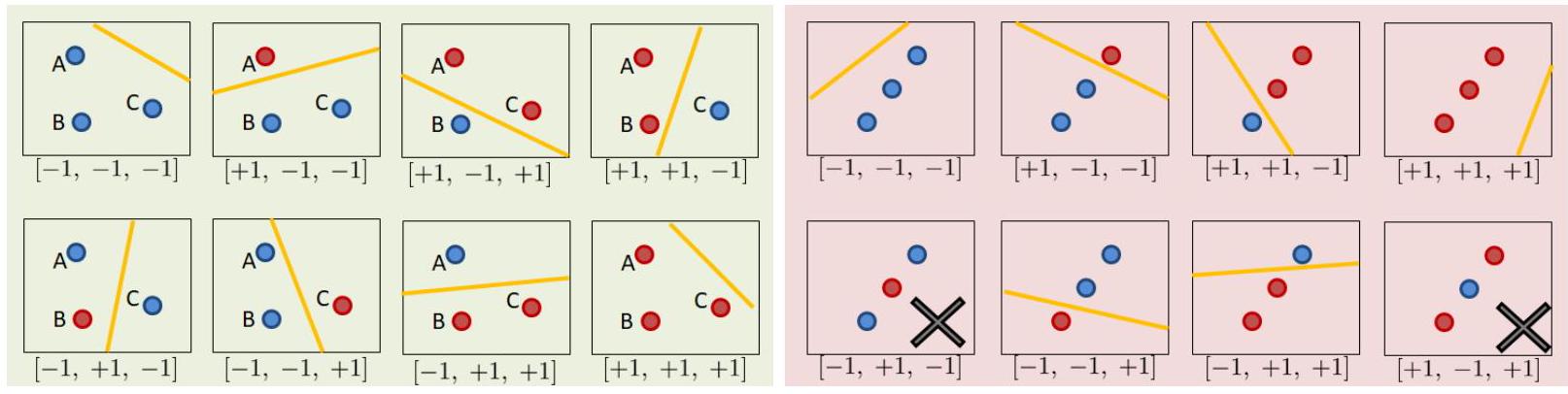
Fig. 19 For a fixed configuration of ${\mathbf{x}}^{(1)},{\mathbf{x}}^{(2)},{\mathbf{x}}^{(3)}$, we can obtain different numbers of dichotomies. Suppose the hypothesis set contains linear models. [Left] There are 8 dichotomies for three data points located not on a line. [Right] When the three data points are located on a line, the number of dichotomies becomes 6.

Now we want to define a quantity that measures the number of dichotomies. This quantity should be universal for any configuration of ${\mathbf{x}}^{(1)},\dots ,{\mathbf{x}}^{(N)}$, and should only be a function of $\mathcal{H}$ and $N$. If we can obtain such quantity, then we will have a way to make a better estimate than $M$. To eliminate the dependency on ${\mathbf{x}}^{(1)},\dots ,{\mathbf{x}}^{(N)}$, we realize that among all the possible configurations of ${\mathbf{x}}^{(1)},\dots ,{\mathbf{x}}^{(N)}$, there exists one that can maximize the size of $\mathcal{H}({\mathbf{x}}^{(1)},\dots ,{\mathbf{x}}^{(N)})$. Define this maximum as the growth function.

Definition 112 (Growth Function)

The growth function for a hypothesis set $\mathcal{H}$ is

(67)$$m_{\mathcal{H}}(N)=\underset{{\mathbf{x}}^{(1)},\dots ,{\mathbf{x}}^{(N)}\in \mathcal{X}}{max}\left|\mathcal{H}({\mathbf{x}}^{(1)},\dots ,{\mathbf{x}}^{(N)})\right|$$

where $|\cdot |$ denotes the cardinality of a set.

Example 22 (Example of Growth Function)

For example, $m_{\mathcal{H}}(3)$ of a linear model is 8 , because if we configure ${\mathbf{x}}^{(1)},{\mathbf{x}}^{(2)},{\mathbf{x}}^{(3)}$ like the ones in the green part of Fig. 19, we will get 8 dichotomies. Of course, if we land on the red case we will get 6 dichotomies only, but the definition of $m_{\mathcal{H}}(3)$ asks for the maximum which is 8. How about $m_{\mathcal{H}}(N)$ when $N=4$ ? It turns out that there are at most 14 dichotomies no matter where we put the four data points ${\mathbf{x}}^{(1)},{\mathbf{x}}^{(2)},{\mathbf{x}}^{(3)},{\mathbf{x}}^{(4)}$.

So what is the difference between $m_{\mathcal{H}}(N)$ and $M$ ? Both are measures of the number of hypotheses. However, $m_{\mathcal{H}}(N)$ is measured from the $N$ training samples in $\mathcal{X}$ whereas $M$ is the number of hypotheses we have in $\mathcal{H}$. The latter could be infinite, the former is upper bounded (at most) $2^N$. Why $2^N$ ? Suppose we have $N$ data points and the hypothesis is binary. Then the set of all dichotomies $\mathcal{H}({\mathbf{x}}^{(1)},\dots ,{\mathbf{x}}^{(N)})$ must be a subset in $\{+1,-1{\}}^N$, and hence there are at most $2^N$ dichotomies:

$$m_{\mathcal{H}}(N)\le 2^N$$

If a hypothesis set $\mathcal{H}$ is able to generate all $2^N$ dichotomies, then we say that $\mathcal{H}$ shatter ${\mathbf{x}}^{(1)},\dots ,{\mathbf{x}}^{(N)}$. For example, a $2\mathrm{D}$ perceptron algorithm is able to shatter 3 data points because $m_{\mathcal{H}}(3)=2^3$. However, the same $2\mathrm{D}$ perceptron algorithm is not able to shatter 4 data points because $m_{\mathcal{H}}(4)=14<2^4$

Definition 113 (Restricted Hypothesis Space)

By only choosing the distinct effective hypotheses on the dataset $S$, we restrict the hypothesis space $\mathcal{H}$ to a smaller subspace that depends on the dataset. We call this new hypothesis space a restricted one:

$${\mathcal{H}}_{\mid S}$$

Ah, what is a consequence of all this? Can we do better with the generalization bound (65) defined in Theorem 63.

The most straight forward step is to replace $M$ by $m_{\mathcal{H}}(N)$ :

$$\hat{\mathcal{R}}(h_S)-\sqrt{\frac{1}{2N}\log \frac{2m_{\mathcal{H}}(N)}{\delta }}\le {\mathcal{R}}_{\mathcal{D}}(h_S)\le \hat{\mathcal{R}}(h_S)+\sqrt{\frac{1}{2N}\log \frac{2m_{\mathcal{H}}(N)}{\delta }}$$

Since we know that

$$m_{\mathcal{H}}(N)\le 2^N$$

a natural attempt is to upper bound $m_{\mathcal{H}}(N)$ by $2^N$.

However, this will not help us because

$$\sqrt{\frac{1}{2N}\log \frac{2m_{\mathcal{H}}(N)}{\delta }}\le \sqrt{\frac{1}{2N}\log \frac{2\left(2^N\right)}{\delta }}=\sqrt{\frac{1}{2N}\log \frac{2^{N+1}}{\delta }}$$

For large $N$ we can approximate $2^{N+1}\approx 2^N$, and so

$$\frac{1}{2N}\log \frac{2^N}{\delta }\approx \frac{N\log 2-\log \delta }{2N}=\frac{\log 2}{2}-\frac{\log \delta }{2N}\to (\log 2)/2.$$

Therefore, as $N\to \mathrm{\infty }$, the error bar will never approach zero but to a constant. This makes the generalization fail.

Furthermore, even though now the restricted hypothesis space ${\mathcal{H}}_{\mid S}$ is “finite”, but $2^N$ is exponential in terms of $N$ and would grow too fast for large datasets, which makes the odds in our inequality go too bad too fast! Is that the best bound we can get on that growth function? Can we do better?

The VC Dimension

Can we find a better upper bound on $m_{\mathcal{H}}(N)$ so that we can send the error bar to zero as $N$ grows? Here we introduce some definitions allows us to characterize the growth function.

Definition 114 (Shattering)

If a hypothesis set $\mathcal{H}$ is able to generate all $2^N$ dichotomies, then we say that $\mathcal{H}$ shatter ${\mathbf{x}}^{(1)},\dots ,{\mathbf{x}}^{(N)}$.

In other words, a set of data points $\mathcal{S}$ is shattered by a hypothesis class $\mathcal{H}$ if there are hypotheses in $\mathcal{H}$ that split $\mathcal{S}$ in all of the $2^{\left|\mathcal{S}\right|}$ possible ways; i.e., all possible ways of classifying points in $\mathcal{S}$ are achievable using concepts in $\mathcal{H}$.

Definition 115 (VC Dimension of $\mathcal{H}$)

The Vapnik-Chervonenkis dimension of a hypothesis set $\mathcal{H}$, denoted by $\mathrm{VCdim}$, is the largest value of $N$ for which $m_{\mathcal{H}}(N)=2^N$.

Example 23 (VC Dimension of a 2D Perceptron)

For example, consider the $2\mathrm{D}$ perceptron algorithm, which has hypothesis $h$ of the following form:

$$\mathrm{sign}\left({\left({\mathbf{x}}^{(n)}\right)}^T\mathbf{w}\right)=y^{(n)}$$

We can start with $N=3$, and gradual increase $N$ until we hit a critical point.

Suppose $N=3$. Recall that $m_{\mathcal{H}}(3)$ is the maximum number of dichotomies that can be generated by a hypothesis set under $N=3$ data points. As we have shown earlier, as long as the 3 data points are not on a straight line, it is possible to draw 8 different dichotomies. If the 3 data points are on a straight line, we can only generate 6 dichotomies. However, since $m_{\mathcal{H}}(3)$ picks the maximum, we have that $m_{\mathcal{H}}(3)=2^3$. Therefore, a 2 D percetpron can shatter 3 data points.

Suppose $N=4$. As we have discussed earlier, if we have $N=4$ data points, there are always 2 dichotomies that cannot be generated by the perceptron algorithm. This implies that the growth function is $m_{\mathcal{H}}(4)=14<2^4$. Since the perceptron algorithm can shatter $N=3$ data points but not $N=4$ data points, the $\mathrm{VC}$ dimension is $\mathrm{VCdim}=3$.

The following animation shows how many ways a linear classifier in 2D can label 3 points (on the left) and 4 points (on the right).

Fig. 20 Image Credit: Machine Learning Theory by Mostafa.

Actually, no linear classifier in 2D can shatter any set of 4 points, not just that set; because there will always be two labellings that cannot be produced by a linear classifier. But why? See the image below.

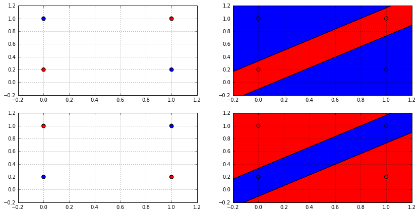
Fig. 21 Image Credit: Machine Learning Theory by Mostafa.

If we arranged the points in a rectangular way like the one in the image, then let the blue dot be class $-1$ and red dot be class $+1$, then there exists no way for a single line (hyperplane if in higher dimensions) to cut the points into two classes.

Moreover, no matter how you arrange these 4 points, whether be it in a line, a rectangle, S-shape or any other arrangements, there will always be at least 2 dichotomies that cannot be generated by a linear classifier. Maybe you could draw some arrangements for yourself and see! Come to think of it, even if you arrange you 4 points in a circle or Z-shape, it will always have 4 “corners” which resemble the 4 points in the image above.

We will soon see how this fact of the impossibility of shattering 4 points is related to the VC dimension of a hypothesis set can be scaled to $N$ data points. And how this can lead us to finding a better bound!

First, let’s find a general formula for the VC dimension of a perceptron algorithm.

Theorem 64 (VC Dimension of a Perceptron)

In general, if we have a high-dimensional perceptron algorithm, we can show this:

Consider the input space $\mathcal{X}={\mathbb{R}}^D\cup \{1\}$ $(\mathbf{x}={[x_1,\dots ,x_D,1]}^T)$. The VC dimension of the perceptron algorithm is

$$\mathrm{VCdim}=D+1$$

Proof. See page 16 of ECE595: Learning Theory

Sauer’s Lemma and Bounding the Growth Function

Now that we have the VC dimension, we can bound the growth function. The following theorem show that $m_{\mathcal{H}}(N)$ is indeed upper bounded by a polynomial of order no greater than $\mathrm{VCdim}$.

Lemma 2 (Sauer’s Lemma)

Let $\mathrm{VCdim}$ be the VC dimension of a hypothesis set $\mathcal{H}$, then

$$\begin{array}{r}{m}_{\mathcal{H}}(N)\le \sum _{i=0}^{\mathrm{VCdim}}\left(\begin{array}{c}N\\ i\end{array}\right)\end{array}$$

Proof. Proof can be found in Theorem $2.4$ of AML’s Learning from Data textbook.

The bound on the growth function provided by Sauer’s Lemma is indeed much better than the exponential one we already have because it is actually a polynomial function.

Using this result, we can show that

$$\begin{array}{r}{m}_{\mathcal{H}}(N)\le \sum _{i=0}^{\mathrm{VCdim}}\left(\begin{array}{c}N\\ i\end{array}\right)\le {\left(\frac{Ne}{\mathrm{VCdim}}\right)}^{\mathrm{VCdim}}\le \mathcal{O}(N^{\mathrm{VCdim}}+1)\end{array}$$

where $e$ is the base of the natural logarithm and $\mathcal{O}$ is the Big-O notation for functions asymptotic (near the limits) behavior.

If we substitute $m_{\mathcal{H}}(N)$ by this upper bound $N^{\mathrm{VCdim}}+1$, then the generalization bound becomes

$$ϵ=\sqrt{\frac{1}{2N}\log \frac{2m_{\mathcal{H}}(N)}{\delta }}\le \sqrt{\frac{1}{2N}\log \frac{2\left(N^{\mathrm{VCdim}}+1\right)}{\delta }}.$$

How do we interpret the VC dimension? The VC dimension can be informally viewed as the effective number of parameters of a model. Higher VC dimension means a more complex model, and hence a more diverse hypothesis set $\mathcal{H}$. Well, we have just shown that for a perceptron or linear classifier, the VC dimension is $D+1$ where $D$ is the dimension of the input space. We have seen that even in 2-dimensional space, if $N=4$ points, then the linear/percepton classifier cannot shatter the points. This is because linear models being linear, cannot model the non-linear decision boundary that can separate the 4 points. However, imagine a complex model like a deep neural network, then you can easily shatter 4 points in 2D space because the decision boundary can be very complex. See the moon dataset in scikit-learn and have a look.

As a result, the growth function $m_{\mathcal{H}}(N)$ will be big. (Think about the number of dichotomies that can be generated by a complex model versus a simple model, and hence the overlap we encounter in the union bound.) There are two scenarios of the VC dimension.

1. $\mathrm{VCdim}<\mathrm{\infty }$. This implies that the generalization error will go to zero as $N$ grows:

   $$ϵ=\sqrt{\frac{1}{2N}\log \frac{2\left(N^{\mathrm{VCdim}}+1\right)}{\delta }}\to 0$$

   as $N\to \mathrm{\infty }$ because $(\log N)/N\to 0$. If this is the case, then the final hypothesis $h_S\in \mathcal{H}$ will generalize. Such generalization result holds independent of the learning algorithm $\mathcal{A}$, independent of the input distribution ${\mathbb{P}}_{\mathcal{D}}$ and independent of the target function $f$. It only depends on the hypothesis set $\mathcal{H}$ and the training examples ${\mathbf{x}}^{(1)},\dots ,{\mathbf{x}}^{(N)}$.

2. $\mathrm{VCdim}=\mathrm{\infty }$. This means that the hypothesis set $\mathcal{H}$ is as diverse as it can be, and it is not possible to generalize. The generalization error will never go to zero.

Are we all set about the generalization bound? It turns out that we need some additional technical modifications to ensure the validity of the generalization bound. We shall not go into the details but just state the result.

Theorem 65 (The VC Generalization Bound)

For any tolerance $\delta >0$

(68)$${\mathcal{R}}_{\mathcal{D}}(h_S)\le {\hat{\mathcal{R}}}_{\mathcal{S}}(h_S)+\sqrt{\frac{\mathcal{8}}{N}\log \frac{\mathcal{4}{m}_{\mathcal{H}}(\mathcal{2}N)}{\delta }}$$

with probability at least $1-\delta$.

To this end, we have more or less answered the question “Is Learning Feasible?”.

Interpretating the Generalization Bound

The VC generalization bound in (68) is universal in the sense that it applies to all hypothesis set $\mathcal{H}$, learning algorithm $\mathcal{A}$, input space $\mathcal{X}$, distribution ${\mathbb{P}}_{\mathcal{D}}$, and binary target function $f$. So can we use the VC generalization bound to predict the exact generalization error for any learning scenario? Unfortunately the answer is no. The VC generalization bound we derived is a valid upper bound but also a very loose upper bound. The loose-ness nature of the generalization bound comes from the following reasons (among others):

• The Hoeffding inequality has a slack. The inequality works for all values of ${\mathcal{R}}_{\mathcal{D}}$. However, the behavior of ${\mathcal{R}}_{\mathcal{D}}$ could be very different at different values, e.g., at 0 or at 0.5. Using one bound to capture both cases will result in some slack.

• The growth function $m_{\mathcal{H}}(N)$ gives the worst case scenario of how many dichotomies are there. If we draw the $N$ data points at random, it is unlikely that we will land on the worst case, and hence the typical value of $m_{\mathcal{H}}(N)$ could be far fewer than $2^N$ even if $m_{\mathcal{H}}(N)=2^N$.

• Bounding $m_{\mathcal{H}}(N)$ by a polynomial introduces further slack.

Therefore, the VC generalization bound can only be used a rough guideline of understanding how well the learning algorithm generalize.

Sample Complexity

Sample complexity concerns about the number of training samples $N$ we need to achieve the generalization performance. Recall from the generalization bound:

$${\mathcal{R}}_{\mathcal{D}}(h_S)\le {\hat{\mathcal{R}}}_{\mathcal{S}}(h_S)+\sqrt{\frac{8}{N}\log \frac{4m_{\mathcal{H}}(2N)}{\delta }}.$$

Fix a $\delta >0$, if we want the generalization error to be at most $ϵ$, we can enforce that

$$\sqrt{\frac{8}{N}\log \frac{4m_{\mathcal{H}}(2N)}{\delta }}\le ϵ$$

Rearranging the terms yields $N\ge \frac{8}{{ϵ}^2}\log \left(\frac{4m_{\mathcal{H}}(2N)}{\delta }\right)$. If we replace $m_{\mathcal{H}}(2N)$ by the VC dimension, then we obtain a similar bound

$$N\ge \frac{8}{{ϵ}^2}\log \left(\frac{4(2N{)}^{\mathrm{VCdim}}+1}{\delta }\right).$$

Example 24 (Sample Complexity)

Suppose $\mathrm{VCdim}=3,ϵ=0.1$ and $\delta =0.1$ (90% confidence). The number of samples we need satisfies the equation

$$N\ge \frac{8}{{0.1}^2}\log \left(\frac{4(2N{)}^3+4}{0.1}\right).$$

If we plug in $N=1000$ to the right hand side, we will obtain

$$N\ge \frac{8}{{0.1}^2}\log \left(\frac{4(2\times 1000{)}^3+4}{0.1}\right)\approx 21,193.$$

If we repeat the calculation by plugging in $N=21,193$, obtain a new $N$, and iterate, we will eventually obtain $N\approx 30,000$. If $\mathrm{VCdim}=4$, we obtain $N\approx 40,000$ samples. This means that every value of $\mathrm{VCdim}$ corresponds to 10,000 samples. In practice, we may require significantly less number of samples. A typical number of samples is approximately $10\times \mathrm{VCdim}$.

Model Complexity

The other piece of information that can be obtained from the generalization bound is how complex the model could be. If we look at the generalization bound, we realize that the error $ϵ$ is a function of $N,\mathcal{H}$ and $\delta$ :

$$\mathcal{R}(h_S)\le \hat{\mathcal{R}}(h_S)+\underset{=ϵ(N,\mathcal{H},\delta )}{\underbrace{\sqrt{\frac{8}{N}\log \frac{4m_{\mathcal{H}}(2N)}{\delta }}}}$$

If we replace $m_{\mathcal{H}}(2N)$ by $(2N{)}^{\mathrm{VCdim}}+1$, then we can write $ϵ(N,\mathcal{H},\delta )$ as

$$ϵ(N,\mathrm{VCdim},\delta )=\sqrt{\frac{8}{N}\log \left(\frac{4((2N{)}^{\mathrm{VCdim}}+1)}{\delta }\right)}$$

The three factors $N,\mathrm{VCdim}$ and $\delta$ have different influence on the error $ϵ$ :

• $\mathrm{VCdim}$ : The VC dimension controls the complexity of the model. As $\mathrm{VCdim}$ grows, the in-sample error $E_{\mathrm{in}}$ drops because large $\mathrm{VCdim}$ implies that we have a more complex model to fit the training data. However, $ϵ$ grows as $\mathrm{VCdim}$ grows. If we have a very complex model, then it would be more difficult to generalize to the out-samples. The trade-off between model complexity and generalization is shown in Fig. 22. The blue curve represents the in-sample error $E_{\mathrm{in}}$ which drops as $\mathrm{VCdim}$ increases. The red curve represents the model complexity which increases as $\mathrm{VCdim}$ increases. The black curve is the out-sample error ${\mathcal{R}}_{\mathcal{D}}$. There exists an optimal model complexity so that ${\mathcal{R}}_{\mathcal{D}}$ is minimized.

• $N$ : A large number of training samples always helps the generalization bound, as reflected by the fact that $ϵ(N,\mathcal{H},\delta )\to 0$ as $N\to \mathrm{\infty }$.

• $\delta$ : The confidence level tells us how harsh we want the generalization to be. If we want a very high confidence interval, e.h_S., $99.99\mathrm{\%}$, then we need a very small $\delta =0.0001$. This will in turn affect the number of training samples $N$ required to achieve the confidence level and the desired error bound.

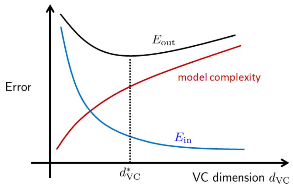
Fig. 22 The VC generalization bound suggests a trade-off between model complexity and generalization. If we use a more complex model, the in-sample error drops but the out-sample error increases. The optimal model complexity is determined when the out-sample error is minimized.

Testing Data

The VC analysis provides us a good guideline to train a model. However, the estimate provided by the $\mathrm{VC}$ analysis is often too loose to provide any accurate prediction of ${\mathcal{R}}_{\mathcal{D}}$. In practice, no one really uses $\mathrm{VC}$ analysis to inform a training process. What is more often used is a testing dataset. The testing dataset

$${\mathcal{S}}_{\text{test }}=\{{\mathbf{x}}^{(1)},\dots ,{\mathbf{x}}^{(Q)}\}$$

contains $Q$ samples drawn from the distribution ${\mathbb{P}}_{\mathcal{D}}(\mathbf{x})$. No testing data ${\mathbf{x}}^{(q)}$ can be in the training dataset ${\mathcal{S}}_{\text{train}}$.

Since in the testing phase the final hypothesis $h_S$ is already determined, we will not run into the same trouble in the training phase where we need to use the Union bound to account for the $M$ candidate hypotheses in $\mathcal{H}$. As a result, the Hoeffding inequality simplifies to

$$\mathbb{P}\{|{\hat{\mathcal{R}}}_{\mathcal{S}}(h_S)-{\mathcal{R}}_{\mathcal{D}}(h_S)|>ϵ\}\le 2e^{-2{ϵ}^{2}Q}$$

and the generalization bound becomes

$${\mathcal{R}}_{\mathcal{D}}(h_S)\le {\hat{\mathcal{R}}}_{\mathcal{S}}(h_S)+\sqrt{\frac{1}{2Q}\log \frac{2}{\delta }}$$

Therefore, as the number of testing samples increases, we can certify the out-sample error by evaluating $\widehat{\mathcal{R}(h_S)}$ using the testing samples.

There are a few reminders about using the testing data:

• The common notion of testing accuracy is ${\hat{\mathcal{R}}}_{\mathcal{S}}(h_S)$, calculated based on the $Q$ testing samples. Therefore, having $\hat{\mathcal{R}}(h_S)$ does not imply that we will generalize well. If we change another testing dataset, $\hat{\mathcal{R}}(h_S)$ will change because it is a numerical value based on empirical sum. What is guaranteed by the generalization bound is that as long as $Q$ is sufficiently large, ${\mathcal{R}}_{\mathcal{D}}(h_S)$ will stay close to ${\hat{\mathcal{R}}}_{\mathcal{S}}(h_S)$ no matter which particular testing dataset we use. There is a variance associated with $\hat{\mathcal{R}}(h_S)$, and this variance is reflected by $\sqrt{\frac{1}{2Q}\log \frac{2}{\delta }}$.

• The testing data has to be used after the hypothesis is determined. If we ever use the testing data as a feedback to re-select the hypothesis, then it is cheating. For example, we cannot train a SVM, submit to a competition website, and mark the misclassified samples to re-design the SVM.

• In principle the generalization bound is improved when we have more testing samples. However, most practical datasets only have training data points and no testing data points. We can partition the training set into training and validation. The proportion of training and validation needs to be carefully chosen. If we allocate too many samples for validation purpose, then we will loose our ability to training a good classifier.

Why must $h$ be fixed and defined before generating the dataset $\mathcal{S}$?

Question and Answer from MathStackExchange.

Some intuition on the difference between a-priori and a-posteriori:

Some intuition on the difference between a-priori and a-posteriori: Let $\{Y_1,...,Y_4\}$ be i.i.d. uniform random variables over $[0,1]$. So for each $m\in \{1,...,4\}$ we have

$$P[Y_m>15/16]=1/16=0.0625$$

A-priori:

Let’s a-priori pick an index $K\in \{1,2,3,4\}$, independent of the $Y_i$ variables and before observing these variables. We can use any mass function $P[K=m]$ for $m\in \{1,2,3,4\}$. What is $P[Y_K>15/16]$? It is still $1/16$ (regardless of the mass function we use) because, by the law of total probability:

$$\begin{array}{r}\begin{array}{rl}P[Y_K>15/16]& =\sum _{m=1}^{4}P[Y_K>15/16|K=m]P[K=m]\\ & =\sum _{m=1}^4\underset{P[Y_m>15/16]}{\underbrace{P[Y_m>15/16|K=m]}}P[K=m]\\ & =\sum _{m=1}^4(1/16)P[K=m]\\ & =1/16\end{array}\end{array}$$

where the equality $P[Y_m>15/16|K=m]=P[Y_m>15/16]$ holds because $Y_m$ is independent of $K$.

A-posteriori:

Now let’s a-posteriori pick the index $K$ associated with the largest $Y_m$ value, so $Y_K=max[Y_1,Y_2,Y_3,Y_4]$. This choice of index $K$ depends on the observed data. Then:

$$\begin{array}{r}\begin{array}{rl}P[Y_K>15/16]& =1-P[Y_1\le 15/16,Y_2\le 15/16,Y_3\le 15/16,Y_4\le 15/16]\\ & =1-(15/16{)}^4\\ & \approx 0.2275\end{array}\end{array}$$

and so this probability is much larger than 1/16, even though $Y_K$ is just one of the $Y_m$ values and we know $P[Y_m>15/16]=1/16$ for all $m\in \{1,...,4\}$.

On the other hand, we know by the union bound that

$$\{Y_K>15/16\}\subseteq {\cup }_{m=1}^4\{Y_m>15/16\}⟹P[Y_K>15/16]\le \sum _{m=1}^{4}P[Y_m>15/16]=1/4$$

and indeed $0.2275\le 1/4$.

Your specific setup

As in my above comment, I believe we need the following extra assumptions: We have a finite set $\mathcal{X}$ and an unknown function $f:\mathcal{X}\to \mathbb{R}$. We are certain that $f$ is one of the $M$ functions in the known set $\{h_1,...,h_M\}$. We have the ability to exactly evaluate the function $f$ one step at a time. However, the set $\mathcal{X}$ is too large so we want to do a probabilistic estimate. Every time step $i$ we independently chose $X_i\in \mathcal{X}$, uniformly over all points in $\mathcal{X}$. We then observe the value of $f(X_i)$ (with no noise).

So for a given function $h_m$ we define ${\varphi }_m$ by:

$${\varphi }_m=P[f(X_i)\ne h_m(X_i)]=\frac{\text{number of points }x\in \mathcal{X}\text{ such that }f(x)\ne h_m(x)}{|\mathcal{X}|}$$

For each $m\in \{1,...,M\}$ define the sequence of indicator functions $\{I_i^{(m)}{\}}_{i=1}^{\mathrm{\infty }}$ by

$$\begin{array}{r}{I}_i^{(m)}=\{\begin{array}{ll}1& \text{ if }{h}_m(X_i)\ne f(X_i)\\ 0& \text{ otherwise}\end{array}\end{array}$$

For any fixed $m\in \{1,...,M\}$ the $\{I_i^{(m)}{\}}_{i=1}^{\mathrm{\infty }}$ indicators are i.i.d. so we can apply Hoeffding. Note that for each individual $m$, Hoeffding is a bound on the following a-priori probability:

$$P[|\frac{1}{N}\sum _{i=1}^N{I}_i^{(m)}-{\varphi }_m|>ϵ]\le 2e^{-2{ϵ}^{2}N}(Eq.1)$$

and it is nice that the bound on the right-hand-side does not depend on the index $m$.

Your specific questions

1. Your first question asks why Hoeffding requires a fixed function $h$ rather than a random function $H$. It is because Hoeffding applies to i.i.d. random variables. If we fix an index $m\in \{1,..,M\}$ then the indicators $\{I_1^{(m)},I_2^{(m)},I_3^{(m)},...\}$ are i.i.d. over the indices $i\in \{1,2,3,...\}$. If we have a random index $K$ then the indicators $\{I_1^{(K)},I_2^{(K)},I_3^{(K)},...\}$ are not necessarily independent because they share a common random index $K$.

2-4) Your remaining questions boil down to the difference between a-priori probability and a-posteriori probability. The Hoeffding bounds in (Eq. 1) are a-priori bounds that hold for all $m\in \{1,...,M\}$. They are bounds on the probability the data behaves in a certain way. That probability (and its bound) is determined without observing the actual data outcome (in the same way that the probability of a fair coin flip being heads is 1/2, and this probability is determined without looking at the outcome of the flip).

If we a-priori pick a random index $K\in \{1,...,M\}$ (before observing the data and independent of the data), then we do not need the union bound:

$$\begin{array}{r}\begin{array}{rl}P[|\frac{1}{N}\sum _{i=1}^N{I}_i^{(K)}-{\varphi }_K|>ϵ]& =\sum _{m=1}^{M}P[|\frac{1}{N}\sum _{i=1}^N{I}_i^{(K)}-{\varphi }_K|>ϵ|K=m]P[K=m]\\ & =\sum _{m=1}^{M}P[|\frac{1}{N}\sum _{i=1}^N{I}_i^{(m)}-{\varphi }_m|>ϵ|K=m]P[K=m]\\ & \stackrel{(a)}{=}\sum _{m=1}^{M}P[|\frac{1}{N}\sum _{i=1}^N{I}_i^{(m)}-{\varphi }_m|>ϵ]P[K=m]\\ & \le \sum _{m=1}^m[2e^{-2{ϵ}^{2}N}]P[K=m]\\ & =2e^{-2{ϵ}^{2}N}\end{array}\end{array}$$

where equality (a) holds because the random index $K$ is independent of the data $\{I_i^{(m)}{\}}_{i=1}^{\mathrm{\infty }}$. So, if we were to a-priori pick a guess function $g$, independent of the data, by just picking a random index, the bound would indeed be $2e^{-2{ϵ}^{2}N}$ rather than $2M{e}^{-2{ϵ}^{2}N}$.

However, if we observe the results of the data and then a-posteriori pick a random index $K\in \{1,...,M\}$, the way we choose might lead us to pick an index that exhibits “atypical” a-posteriori sample paths. So the equality (a) in the above chain of equalities does not necessarily hold for such picks. We need to be more careful by using the union bound.

---

Exercise: Code up hoefdding inequality with plot.

Further Readings

This is a difficult topic to learn. I recommend the following resources:

• Mohri, Mehryar, Afshin Rostamizadeh, and Ameet Talwalkar. Foundations of Machine Learning. MIT press, 2012.

• Shalev-Shwartz, Shai, and Shai Ben-David. Understanding Machine Learning: From Theory to Algorithms. Cambridge University Press, 2014.

• Abu-Mostafa, Y. S., Magdon-Ismail, M., & Lin, H. (2012). Learning from Data: A Short Course.

• Mitchell, Tom M. Machine learning. Vol. 1. , bk. 9. : McGraw-hill New York, 1997.

• Nathaniel Dake: Probability Inequalities

• ECE595: Learning Theory

• ECE595: Learning Theory Lectures (Part 3)

• Mostafa Samir: Machine Learning Theory

• Zhang Wei: Learning Theory

• Nathaniel Dake: Probability Inequalities

• Prof chan’s video lectures ECE595: Learning Theory

• https://d2l.ai/chapter_linear-classification/generalization-classification.html

• 1. Why is Hoeffding’s inequality invalid if we use $h_S$ instead of $h$?

• 2. Why is Hoeffding’s inequality invalid if we use $h_S$ instead of $h$?

• 3. Why is Hoeffding’s inequality invalid if we use $h_S$ instead of $h$?

• 4. Why is Hoeffding’s inequality invalid if we use $h_S$ instead of $h$?

• Why do we need to use Union Bound?

• Union Bound Example

• Generalization in Classification

• CMU 10-601: Machine Learning

• Why is the Hoeffding’s Inequality correct in Machine Learning?

---

1

Sometimes $f$ is denoted as $\mathcal{c}$, the concept function.