\[ \newcommand{\ytrue}{\mathbf{y_{\textbf{true}}}} \newcommand{\yprob}{\mathbf{y_{\textbf{prob}}}} \newcommand{\y}{\mathbf{y}} \newcommand{\x}{\mathbf{x}} \]

Cross Entropy Loss#

Intuition#

We need to make sense of entropy in the form of a loss function, we have to just enhance our thinking a little.

We define our target to be a one-hot encoded vector of class 0 and 1.

target = [0, 1]

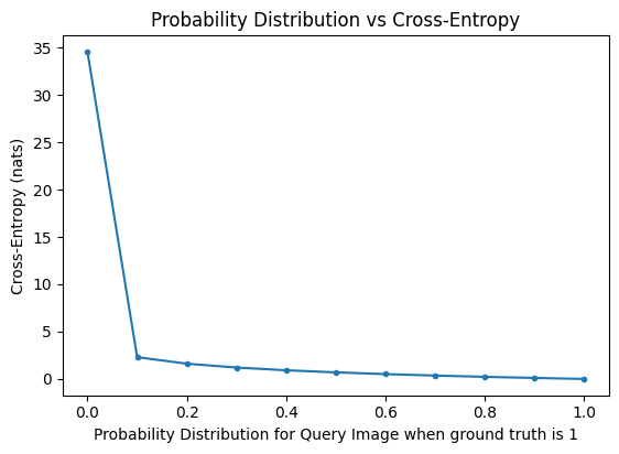
Intuitively, take the cat vs dog binary classification again, we made 11 predictions for ONLY ONE query image using different model, and find that after going through many layers, the softmax predictions on the logits are as such:

[
    [0.0, 1.0],
    [0.1, 0.9],
    [0.2, 0.8],
    [0.3, 0.7],
    [0.4, 0.6],
    [0.5, 0.5],
    [0.6, 0.4],
    [0.7, 0.3],
    [0.8, 0.2],
    [0.9, 0.1],
    [1.0, 0.0],
]

where the first index corresponds to the logits of class 0 and second index corresponds to the logits of class 1.

For example, [1, 0] means the model is 100 percent confident the prediction is a class 0 (cat), and obviously we need to punish the model for spitting nonsense like this.

As we can see in the binary_cross_entropy function below, we only need to add up two things. And note that we are hinging on class 1 and therefore y_true[0] * log(y_pred[0]+eps) goes to 0 as we are just relying on our feedback of probability of class 1.

And in our graph, we can see that as predictions gets more wrong, meaning to say, if the query image is a dog, but our predictions is [1, 0], which says it is a cat, our entropy loss will blow up to very high because

y_true[1] * log(y_pred[1]+eps) -> 1 * log(1+eps) -> almost infinity

Note again we do not calculate for class 0 because

We one-hot encoded.
We only look at class 1’s probability and that’s enough as we can deduce class 0’s probability anyways.

And conversely, note how the entropy loss goes to 0 if our prediction is say [0, 1]. In general, as our probability for the query image gets close to 1, or in agreement with our class, then our entropy loss becomes smaller.

import numpy as np
import torch
import torch.nn.functional as F
import matplotlib.pyplot as plt

torch.__version__

'1.13.0+cu117'

def torch_to_np(tensor: torch.Tensor) -> np.ndarray:
    """Convert a PyTorch tensor to a numpy array.

    Args:
        tensor (torch.Tensor): The PyTorch tensor to convert.

    Returns:
        np.ndarray: The converted numpy array.
    """
    return tensor.detach().cpu().numpy()

def compare_equality_two_tensors(
    tensor1: torch.Tensor, tensor2: torch.Tensor
) -> bool:
    """Compare two PyTorch tensors for equality.

    Args:
        tensor1 (torch.Tensor): The first PyTorch tensor to compare.
        tensor2 (torch.Tensor): The second PyTorch tensor to compare.

    Returns:
        bool: Whether the two tensors are equal.
    """
    if torch.all(torch.eq(tensor1, tensor2)):
        return True
    return False


def compare_closeness_two_tensors(
    tensor1: torch.Tensor,
    tensor2: torch.Tensor,
    epsilon: float,
    *args,
    **kwargs
) -> bool:
    """Compare two PyTorch tensors for closeness.

    Args:
        tensor1 (torch.Tensor): The first PyTorch tensor to compare.
        tensor2 (torch.Tensor): The second PyTorch tensor to compare.
        epsilon (float): The epsilon value to use for closeness.

    Returns:
        bool: Whether the two tensors are close.
    """
    if torch.allclose(tensor1, tensor2, atol=epsilon, *args, **kwargs):
        return True
    return False

Cross-Entropy as a Loss Function#

Cross-Entropy Setup#

We first understand the idea and intuition of Cross-Entropy Loss on one single example. Consider a dataset of cat (class 0) and dogs (class 1) where after one hot encoding we have class 0 to be $[1, 0]$ and class 1 to be $[0, 1]$.

We are given the following:

$\mathcal{S}$: The dataset $\mathcal{S}$ generated from the underlying distribution $\mathbb{P}_{\mathcal{D}}$.
$\mathbf{X}$: This is a $2 \times 3 \times 224 \times 224$ tensor of the shape $B \times C \times H \times W$. This can be understood as 2 RGB images of size 224.
$\mathbf{y}$: This is the corresponding ground truth one-hot encoded matrix, we have cat, dog and pig respectively (3 classes):

\[\begin{split} \ytrue = \begin{bmatrix} 1 & 0 & 0 \\ 0 & 0 & 1 \end{bmatrix} \end{split}\]
$\mathbf{x}_i$: We represent each $x_{i}$ as the $i$-th image. This can be a random variable. Image 1 is a cat, and Image 2 is a pig.
$\mathbf{y}_i$: The corresponding label for the $i$-th sample/image, for sample 1, it is $\begin{bmatrix} 1 & 0 & 0 \end{bmatrix}$.
$P$: The probability distribution for the ground truth target - when it is $[1, 0, 0]$, one can understand it as the distribution where cat’s probability is 1, and dog’s probability is 0 and pig 0.
$Q$: The probability distribtion of the estimate on the $\mathbf{x}_i$, which is say, $[0.9, 0.01, 0.09]$.

X = torch.zeros(size=(2, 3, 224, 224), dtype=torch.float32)
y_true = torch.tensor([0, 2], dtype=torch.long)
y_true_ohe = torch.tensor([[1, 0, 0], [0, 0, 1]], dtype=torch.long)
print(y_true_ohe)
compare_equality_two_tensors(y_true_ohe, torch.nn.functional.one_hot(y_true, num_classes=3))

tensor([[1, 0, 0],
        [0, 0, 1]])

True

Z Logits#

Then we have the following, assume a hypothesis $h_{\theta}(\mathcal{X})$ on the dataset $\mathcal{X}$ and it outputs logits of the form, note that we are passing in inputs of shape $(2, 3, 224, 224)$ but after some transformations we have the logits to be shape $(2, 3)$:

z_logits: $$\textbf{z_logits} = \begin{bmatrix} 1 & 2 & 3 \\ 2 & 4 & 6 \end{bmatrix}$$

z_logits = torch.tensor([[1, 2, 3], [2, 4, 6]], dtype=torch.float32)
print(z_logits)

tensor([[1., 2., 3.],
        [2., 4., 6.]])

Softmax1 #

The softmax function takes as input a vector $\mathbf{z}$ of $K$ real numbers, and normalizes it into a probability distribution consisting of $K$ probabilities proportional to the exponentials of the input numbers. That is, prior to applying softmax, some vector components could be negative, or greater than one; and might not sum to 1; but after applying softmax, each component will be in the interval of 0 and 1, and the components will add up to 1, so that they can be interpreted as probabilities. Furthermore, the larger input components will correspond to larger probabilities.

The standard (unit) softmax function

\[\sigma : \mathbb{R}^K\to (0,1)^K\]

is defined when $K$ is greater than one by the formula:

\[ \sigma(\mathbf{z})_i = \frac{e^{z_i}}{\sum_{j=1}^K e^{z_j}} \ \ \ \ \text{ for } i = 1, \dotsc , K \text{ and } \mathbf z=(z_1,\dotsc,z_K) \in \mathbb{R}^K \]

In linear algebra notation, the $\sigma$ soft(arg)max function takes in a real vector $\mathbf{z}$ from the $K$ dimensional space, indicating that the vector $\mathbf{z} \in \mathbb{R}^K$ has $K$ number of elements, and maps to the $K$ dimensional 0-1 space, which is also a vector of $K$ elements; in other words, given an input vector $\mathbf{z} \in \mathbb{R}^K$, the soft(arg)max maps it to $\sigma(\mathbf{z}) \in (0,1)^K$.

Now we break down what the soft(arg)max function actually does. It applies the standard exponential function to each element $z_i$ of the input vector $\mathbf{z}$ and normalizes these values by dividing by the sum of all these exponentials; this normalization ensures that the sum of the components of the output vector $\sigma(\mathbf z)$ is 1.

After applying softmax to the logits we have:

y_prob = z_softargmax: $$\yprob = \textbf{z_softargmax} = \begin{bmatrix} 0.09 & 0.2447 & 0.6652 \\ 0.0159 & 0.1173 & 0.8668\end{bmatrix}$$

def compute_softargmax(z: torch.Tensor) -> torch.Tensor:
    """Compute the softargmax of a PyTorch tensor.

    Args:
        z (torch.Tensor): The PyTorch tensor to compute the softargmax of.

    Returns:
        torch.Tensor: The softargmax of the PyTorch tensor.
    """

    # the output matrix should be the same size as the input matrix
    z_softargmax = torch.zeros(size=z.size(), dtype=torch.float32)

    for row_index, each_row in enumerate(z):
        denominator = torch.sum(torch.exp(each_row))
        for element_index, each_element in enumerate(each_row):
            z_softargmax[row_index, element_index] = (
                torch.exp(each_element) / denominator
            )

    assert compare_closeness_two_tensors(
        z_softargmax, torch.nn.Softmax(dim=1)(z), 1e-15
    )
    return z_softargmax

z_softargmax = compute_softargmax(z_logits)
print(z_softargmax)

tensor([[0.0900, 0.2447, 0.6652],
        [0.0159, 0.1173, 0.8668]])

Categorical Cross Entropy Loss#

We will start with this because the Binary Cross Entropy Loss is merely a special case of this. Finding the full compact formula for this took me a while since most tutorials cover the binary case.

Given $N$ samples, and $C$ classes, the Categorical Cross Entropy Loss is the average loss across $N$ samples, given by:

\[\textbf{CE}(\ytrue, \yprob) = -\dfrac{1}{N}\sum_{i=1}^N\sum_{c=1}^C \mathbb{1}_{\y_{i} \in C_c} \log\left(p_{\textbf{model}}[\y_i \in C_c]\right)\]

where

The outer loop $i$ iterates over $N$ observations/samples.
The inner loop $c$ iterates over $C$ classes.
$\y_i$ represents the true label (in this formula it should be one-hot encoded) of the $i$-th sample.
$\mathbb{1}_{y_{i} \in C_c}$ is an indicator function, simply put, for sample $i$, if the true label $\y_i$ belongs to the $c$-th category, then we assign a $1$, else $0$. We can see it with an example later.
$\left(p_{\textbf{model}}[\y_i \in C_c]\right)$ means the probability predicted by the model for the $i$-th observation that belongs to the $c$-th class category.

\[\begin{split} \ytrue = \begin{bmatrix} 1 & 0 & 0 \\ 0 & 0 & 1 \end{bmatrix} \end{split}\]

\[\begin{split} \textbf{z_logits} = \begin{bmatrix} 1 & 2 & 3 \\ 2 & 4 & 6 \end{bmatrix} \end{split}\]

\[\begin{split} \yprob = \textbf{z_softargmax} = \begin{bmatrix} 0.09 & 0.2447 & 0.6652 \\ 0.0159 & 0.1173 & 0.8668\end{bmatrix} \end{split}\]

We first look at the first sample, index $i = 1$:
- We have the one-hot encoded label for first sample to be $\y_1 = \begin{bmatrix} 1 & 0 & 0 \end{bmatrix}$. This means the label is a cat since the sequence is cat, dog and pig, and thus 1, 0, 0 corresponds to cat 1, dog 0 and pig 0.
- We have the one-hot encoded probability predicted by the model for the first sample to be $\hat{\y_1} = \begin{bmatrix} 0.09 & 0.2447 & 0.6652 \end{bmatrix}$. This means the probability associated with this sample $1$ is probability of a cat from the model is $9\%$, a dog $24.47\%$ and a pig $66.52\%$.

With these information, we go on to the first outer loop’s content:
- $\sum_{c=1}^C \mathbb{1}_{\y_{i} \in C_c} \log\left(p_{\textbf{model}}[\y_i \in C_c]\right)$
- We are looping through the classes, which in this case is loop from $c=1$ to $c=3$ since $C=3$ (3 classes).
- $c = 1$:
  - $\mathbb{1}_{\y_{i} \in C_c} = \mathbb{1}_{\y_{1} \in C_1}$: The true label for the first sample is actually the first class, and hence belongs to the $c=1$ category, so our indicator function returns me a $1$.
  - $\log\left(p_{\textbf{model}}[\y_i \in C_c]\right) = \log\left(p_{\textbf{model}}[\y_1 \in C_1]\right)$: Applies the log function (natural log here) to the each probability associated with the class. So in this case, since $c=1$, we apply the log function to the first entry $0.09$. We get $\log(0.09) = -2.4079$
- $c = 2$:
  - $\mathbb{1}_{\y_{i} \in C_c} = \mathbb{1}_{\y_{1} \in C_2}$: The true label for the first sample is actually the first class, and hence does not belong to the $c=2$ category, so our indicator function returns me a $0$.
  - Regardless, the log of this probability is $\log(0.2447) = -1.4076$
- $c = 3$:
  - $\mathbb{1}_{\y_{i} \in C_c} = \mathbb{1}_{\y_{1} \in C_3}$: The true label for the first sample is actually the first class, and hence does not belong to the $c=3$ category, so our indicator function returns me a $0$.
  - Regardless, the log of this probability is $\log(0.6652) = -0.4076$
- Lastly, we sum them up and get $-2.4076 + 0 + 0 = -2.4076$, note here we only have the first entry! The second and third are $0$.
- In code, this corresponds to the following:
```
    # loop = 1
    current_sample_loss = 0
    for each_y_true_element, each_y_prob_element in zip(
        each_y_true_one_hot_vector, each_y_prob_one_hot_vector
    ):
        # Indicator Function
        if each_y_true_element == 1:
            current_sample_loss += -1 * torch.log(each_y_prob_element)
        else:
            current_sample_loss += 0
```
- Bonus: If you realize this is just a vector dot product: $\begin{bmatrix} 1 & 0 & 0 \end{bmatrix} \cdot \log\left(\begin{bmatrix} 0.09 \\ 0.2447 \\ 0.6652 \end{bmatrix}\right) = \begin{bmatrix} 1 & 0 & 0 \end{bmatrix} \cdot \left(\begin{bmatrix} -2.4076 \\ -1.4076 \\ -0.4076 \end{bmatrix}\right) = -2.4076$

We now look at the second sample, index $i = 2$:
- We have the one-hot encoded label for second sample to be $\y_2 = \begin{bmatrix} 0 & 0 & 1 \end{bmatrix}$. This means the label is a pig since the sequence is cat, dog and pig, and thus 0, 0, 1 corresponds to cat 0, dog 0 and pig 1.
- We have the one-hot encoded probability predicted by the model for the second sample to be $\hat{\y_2} = \begin{bmatrix} 0.0159 & 0.1173 & 0.8868 \end{bmatrix}$. This means the probability associated with this sample $2$ is probability of a cat from the model is $1.59\%$, a dog $11.73\%$ and a pig $88.68\%$.

With these information, we go on to the second outer loop’s content:
- $\sum_{c=2}^C \mathbb{1}_{\y_{i} \in C_c} \log\left(p_{\textbf{model}}[\y_i \in C_c]\right)$
- $c = 2$:
  - $\mathbb{1}_{\y_{i} \in C_c} = \mathbb{1}_{\y_{2} \in C_1}$: The true label for the second sample is actually the third class, and hence belongs to the $c=3$ category, so our indicator function returns me a $0$.
  - $\log\left(p_{\textbf{model}}[\y_i \in C_c]\right)$: Applies the log function (natural log here) to the each probability associated with the class. So in this case, since $c=1$, we apply the log function to the first entry $0.0159$. We get $\log(0.0159) = -4.1429$
- $c = 2$:
  - $\mathbb{1}_{\y_{i} \in C_c} = \mathbb{1}_{\y_{2} \in C_2}$: The true label for the second sample is actually the third class, and hence does not belong to the $c=2$ category, so our indicator function returns me a $0$.
  - Regardless, the log of this probability is $\log(0.1173) = -2.1429$
- $c = 3$:
  - $\mathbb{1}_{\y_{i} \in C_c} = \mathbb{1}_{\y_{2} \in C_3}$: The true label for the second sample is actually the third class, so our indicator function returns me a $1$.
  - The log of this probability is $\log(0.6652) = -0.1429$
- Lastly, we sum them up and get $0 + 0 + (-0.1429) = -0.1429$, note here we only have the third entry! The first and second entries are $0$.
- In code, this corresponds to the following:
```
    # loop = 2
    current_sample_loss = 0
    for each_y_true_element, each_y_prob_element in zip(
        each_y_true_one_hot_vector, each_y_prob_one_hot_vector
    ):
        # Indicator Function
        if each_y_true_element == 1:
            current_sample_loss += -1 * torch.log(each_y_prob_element)
        else:
            current_sample_loss += 0
```
- Bonus: If you realize this is just a vector dot product: $\begin{bmatrix} 0 & 0 & 1 \end{bmatrix} \cdot \log\left(\begin{bmatrix} 0.0159 \\ 0.1173 \\ 0.8868\end{bmatrix}\right) = \begin{bmatrix} 0 & 0 & 1 \end{bmatrix} \cdot \left(\begin{bmatrix} -4.1429 \\ -2.1429 \\ -0.1429 \end{bmatrix}\right) = -0.1429$

To summarize the whole process:

set all_samples_loss = 0
Start Outer Loop:
- loop over first sample i = 1 (actually index is 0 in python):
  - set current_sample_loss = 0
  - loop over $C=3$ classes:
    - when $c = 1$: the loss associated is $-2.4076$. Add this to current_sample_loss.
    - when $c = 2$: the loss associated is $0$. Add this to current_sample_loss.
    - when $c = 3$: the loss associated is $0$. Add this to current_sample_loss.
  - end first loop: update all_samples_loss by adding current_sample_loss to be all_samples_loss = -2.4076.
- loop over second sample i = 2 (actually index is 1 in python):
  - set current_sample_loss = 0
  - loop over $C=3$ classes:
    - when $c = 1$: the loss associated is $0$. Add this to current_sample_loss.
    - when $c = 2$: the loss associated is $0$. Add this to current_sample_loss.
    - when $c = 3$: the loss associated is $-0.1429$. Add this to current_sample_loss.
  - end second loop: update all_samples_loss by adding current_sample_loss to be all_samples_loss = -2.4076 + (-0.1429) = -2.5505.
End all loops: You can multiply by negative $-1$ to make all_samples_loss positive and get all_samples_average_loss = all_samples_loss / num_of_samples = 2.5505 / 2 = 1.2753.

def compute_categorical_cross_entropy_loss(
    y_true: torch.Tensor, y_prob: torch.Tensor
) -> torch.Tensor:
    """Compute the categorical cross entropy loss between two PyTorch tensors.

    Args:
        y_true (torch.Tensor): The true labels.
        y_prob (torch.Tensor): The predicted labels.

    Returns:
        torch.Tensor: The categorical cross entropy loss.
    """

    all_samples_loss = 0
    for each_y_true_one_hot_vector, each_y_prob_one_hot_vector in zip(
        y_true, y_prob
    ):
        current_sample_loss = 0
        for each_y_true_element, each_y_prob_element in zip(
            each_y_true_one_hot_vector, each_y_prob_one_hot_vector
        ):
            # in case y_prob has elements that is 0 or very small, then torch.log(0) might go to -inf
            each_y_prob_element = torch.clamp(each_y_prob_element, min=1.0e-20, max=1.0-1.0e-20, out=None) 
            # Indicator Function
            if each_y_true_element == 1:
                current_sample_loss += -1 * torch.log(each_y_prob_element)
            else:
                current_sample_loss += 0

        all_samples_loss += current_sample_loss

    all_samples_average_loss = all_samples_loss / y_true.shape[0]
    return all_samples_average_loss

Using Dot Product to Calculate#

\[\begin{split} \begin{aligned} \textbf{CE}(\ytrue, \yprob) &= -\dfrac{1}{N}\sum_{i=1}^N\sum_{c=1}^C \mathbb{1}_{\y_{i} \in C_c} \log\left(p_{\textbf{model}}[\y_i \in C_c]\right)\\ &= \textbf{SUM}\left[\textbf{diag}\left(\ytrue \cdot -\log(\yprob)^\top\right)\right] \end{aligned}\end{split}\]

We can easily see

\[\begin{split} \ytrue = \begin{bmatrix} 1 & 0 & 0 \\ 0 & 0 & 1 \end{bmatrix} \end{split}\]

\[\begin{split} \textbf{z_logits} = \begin{bmatrix} 1 & 2 & 3 \\ 2 & 4 & 6 \end{bmatrix} \end{split}\]

\[\begin{split} \yprob = \textbf{z_softargmax} = \begin{bmatrix} 0.09 & 0.2447 & 0.6652 \\ 0.0159 & 0.1173 & 0.8668\end{bmatrix} \end{split}\]

\[\begin{split}\log(\yprob) = \begin{bmatrix} 2.4076 & 1.4076 & 0.4076 \\ 4.1429 & 2.1429 & 0.1429 \end{bmatrix}\end{split}\]

\[\begin{split} \ytrue \cdot -\log(\yprob)^\top = \begin{bmatrix} 1 & 0 & 0 \\ 0 & 0 & 1 \end{bmatrix} \cdot \begin{bmatrix} 2.4076 & 4.1429 \\ 1.4076 & 2.1429 \\ 0.4076 & 0.1429 \end{bmatrix} = \begin{bmatrix} 2.4076 & 4.1429 \\ 0.4076 & 0.1429 \end{bmatrix} \end{split}\]

The matrix $\ytrue \cdot -\log(\yprob)^\top$ diagonals are what we need, where we sum them up and divide by the number of samples. That is $\frac{2.4076+0.1429}{2} = \frac{2.5505}{2} = 1.2753$.

This makes sense because the one hot encoded $\ytrue$ vector guarantees only the indicator functions 1 gets activated and the rest gets zeroed out. Furthermore, we are only interested in the diagonal of the matrix as we are only interested in the dot product between the $i$-th row and the $i$-th column of $\ytrue$ and $-\log(\yprob)^\top$ respectively.

def compute_categorical_cross_entropy_loss_dot_product(
    y_true: torch.Tensor, y_prob: torch.Tensor
) -> torch.Tensor:
    """Compute the categorical cross entropy loss between two PyTorch tensors using dot product.

    Args:
        y_true (torch.Tensor): The true labels in one-hot form.
        y_prob (torch.Tensor): The predicted labels in one-hot form.

    Returns:
        torch.Tensor: The categorical cross entropy loss.
    """
    m = torch.matmul(y_true.float(), torch.neg(torch.log(y_prob.float()).T))
    all_loss_vector = torch.diagonal(m, 0)
    all_loss_sum = torch.sum(all_loss_vector, dim=0)
    average_loss = all_loss_sum / y_true.shape[0]
    return average_loss

compute_categorical_cross_entropy_loss(y_true = y_true_ohe, y_prob = compute_softargmax(z_logits))

tensor(1.2753)

compute_categorical_cross_entropy_loss_dot_product(y_true = y_true_ohe, y_prob = compute_softargmax(z_logits))

tensor(1.2753)

torch.nn.CrossEntropyLoss()(z_logits, y_true)

tensor(1.2753)

z_logits, z_softargmax, y_true_ohe, y_true

(tensor([[1., 2., 3.],
         [2., 4., 6.]]),
 tensor([[0.0900, 0.2447, 0.6652],
         [0.0159, 0.1173, 0.8668]]),
 tensor([[1, 0, 0],
         [0, 0, 1]]),
 tensor([0, 2]))

(-1 * torch.log(z_softargmax)).T

tensor([[2.4076, 4.1429],
        [1.4076, 2.1429],
        [0.4076, 0.1429]])

m = y_true_ohe.float().matmul((-1 * torch.log(z_softargmax)).T)
m

tensor([[2.4076, 4.1429],
        [0.4076, 0.1429]])

torch.diagonal(m, 0).sum()

tensor(2.5505)

Stackoverflow answer#

def cross_entropy(y_true: np.ndarray, y_pred: np.ndarray, epsilon: float = 1e-12):
    """
        https://stackoverflow.com/questions/47377222/what-is-the-problem-with-my-implementation-of-the-cross-entropy-function
        Computes cross entropy between targets (encoded as one-hot vectors)
        and y_pred.
        Input: y_pred (N, k) ndarray
               y_true (N, k) ndarray
        Returns: scalar
        predictions = np.array([[0.25,0.25,0.25,0.25],
                            [0.01,0.01,0.01,0.96]])
    targets = np.array([[0,0,0,1],
                       [0,0,0,1]])
                       ans = 0.71355817782  #Correct answer
    x = cross_entropy(predictions, targets)
    print(np.isclose(x,ans))
    """
    y_pred = np.clip(y_pred, epsilon, 1.0 - epsilon)
    # take note that y_pred is of shape 1 x n_samples as stated in our framework
    n_samples = y_pred.shape[1]

    # cross entropy function
    cross_entropy_function = y_true * np.log(y_pred) + (1 - y_true) * np.log(1 - y_pred)
    # cross entropy function here is same shape as y_true and y_pred since we are
    # just performing element wise operations on both of them.
    assert cross_entropy_function.shape == (1, n_samples)

    # we sum up all the loss for each individual sample
    total_cross_entropy_loss = -np.sum(cross_entropy_function, axis=1)
    assert total_cross_entropy_loss.shape == (1,)

    # we then average out the total loss across m samples, but we squeeze it to
    # make it a scalar; squeeze along axis = None since there is no column axix
    average_cross_entropy_loss = np.squeeze(total_cross_entropy_loss / n_samples, axis=None)

    # cross_entropy_loss = -np.sum(y_true * np.log(y_pred)) / n_samples
    # print(np.isclose(average_cross_entropy_loss, cross_entropy_loss))
    return average_cross_entropy_loss

cross_entropy(y_true=np.asarray([[0, 1]]), y_pred=np.asarray([[0.01, 0.99]]))

array(0.01005034)

MachineLearningMastery example#

from math import log

# calculate cross-entropy
def cross_entropy(p, q, ets=1e-15):
    return -sum([p[i]*log(q[i]+ets) for i in range(len(p))])

def binary_cross_entropy(y_true, y_pred, eps=1e-15):
    return -(y_true[0] * log(y_pred[0]+eps) + y_true[1] * log(y_pred[1]+eps))

# define the target distribution for two events
target = [0.0, 1.0]
# define probabilities for the first event
probs = [
    [0.0, 1.0], # cat is 0% and dog is 100% confidence
    [0.1, 0.9],
    [0.2, 0.8],
    [0.3, 0.7],
    [0.4, 0.6],
    [0.5, 0.5],
    [0.6, 0.4],
    [0.7, 0.3],
    [0.8, 0.2],
    [0.9, 0.1],
    [1.0, 0.0],
]

# create probability distributions for the two events
# dists = [[1.0 - p, p] for p in probs]
# calculate cross-entropy for each distribution
ents = [binary_cross_entropy(y_true=target, y_pred=d) for d in probs]
# plot probability distribution vs cross-entropy
plt.plot([p[1] for p in probs], ents, marker='.')
plt.title('Probability Distribution vs Cross-Entropy')
#pyplot.xticks([1-p for p in probs], ['[%.1f,%.1f]'%(d[0],d[1]) for d in dists], rotation=70)
plt.subplots_adjust(bottom=0.2)
plt.xlabel('Probability Distribution for Query Image when ground truth is 1')
plt.ylabel('Cross-Entropy (nats)')
plt.show()

../../../_images/9428b4157bb1556c865973c6369079c4c5160aa36b214208fa57750e711001e9.png

Probability & Statistics

Cross Entropy Loss

Contents

Cross Entropy Loss#

Intuition#

Cross-Entropy as a Loss Function#

Cross-Entropy Setup#

Z Logits#

Softmax1 #

Categorical Cross Entropy Loss#

Using Dot Product to Calculate#

Stackoverflow answer#

MachineLearningMastery example#

Further Readings#

Probability & Statistics

Cross Entropy Loss

Contents

Cross Entropy Loss#

Intuition#

Cross-Entropy as a Loss Function#

Cross-Entropy Setup#

Z Logits#

Softmax1#

Categorical Cross Entropy Loss#

Using Dot Product to Calculate#

Stackoverflow answer#

MachineLearningMastery example#

Further Readings#

Softmax1 #