Concept

Joint PMF (Discrete Random Variables)

Definition 59 (Joint PMF)

Let \(X\) and \(Y\) be two discrete random variables with sample spaces \(\S_X\) and \(\S_Y\) respectively.

Let \(\eventA = \lset X(\omega) = x, Y(\xi) = y \rset\) be any event in the sample space \(\S_X \times \S_Y\).

The joint probability mass function (joint PMF) of \(X\) and \(Y\) of the event \(\eventA\) is defined as a function \(\pmfjointxy(x, y)\) that can be summed to yield a probability

\[\begin{split} \begin{aligned} \pmfjointxy(x, y) &= \P \lsq X = x \wedge Y = y \rsq \\ &= \P \lsq (\omega, \xi) ~ \lvert ~ X(\omega) = x \wedge Y(\xi) = y \rsq \\ &= \sum_{\omega \in \S_X} \sum_{\xi \in \S_Y} \P \lsq (\omega, \xi) ~ \lvert ~ X(\omega) = x \wedge Y(\xi) = y \rsq \end{aligned} \end{split}\]

where \(\P\) is the probability function defined over the probability space \(\pspace\).

Remark 8 (Joint PMF)

Consider \(\eventA = \lset X(\omega) = x, Y(\xi) = y \rset\). Then \(\eventA\) is an event in the sample space \(\S_X \times \S_Y\). The size of the event \(\eventA\) is

\[ \P \lsq \eventA \rsq = \sum_{(x, y) \in \eventA} \pmfjointxy(x, y) \]

where the sum is over all the possible outcomes in \(\eventA\).

Pictorially represented below in Fig. 8, the joint PMF is a 2D array of impulses.

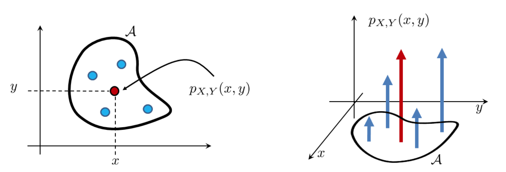
Fig. 8 A joint PMF for a pair of discrete random variables consists of an array of impulses. To measure the size of the event \(\eventA\), we sum all the impulses inside \(\eventA\). Image Credit: [Chan, 2021].

Joint PDF (Continuous Random Variables)

Definition 60 (Joint PDF)

Let \(X\) and \(Y\) be two continuous random variables with sample spaces \(\S_X\) and \(\S_Y\) respectively.

Let \(\eventA \subseteq \S_X \times \S_Y\) be any event in the sample space \(\S_X \times \S_Y\).

Then, the joint PDF of \(X\) and \(Y\) of the event \(\eventA\) is defined as a function \(\pdfjointxy(x, y)\) that can be integrated to yield a probability

(29)\[ \P \lsq \eventA \rsq = \int_{\eventA} \pdfjointxy(x, y) \, dx \, dy \]

Remark 9 (Joint PDF)

Pictorially, we can view \(f_{X, Y}\) as a 2D function where the height at a coordinate \((x, y)\) is \(f_{X, Y}(x, y)\), as can be seen from Fig. 9. To compute the probability that \((X, Y) \in \mathcal{A}\), we integrate the function \(f_{X, Y}\) with respect to the area covered by the set \(\mathcal{A}\). For example, if the set \(\mathcal{A}\) is a rectangular box \(\mathcal{A}=[a, b] \times[c, d]\), then the integration becomes [Chan, 2021]

\[\begin{split} \begin{aligned} \mathbb{P}[\mathcal{A}] & =\mathbb{P}[a \leq X \leq b, \quad c \leq Y \leq d] \\ & =\int_c^d \int_a^b f_{X, Y}(x, y) d x d y \end{aligned} \end{split}\]

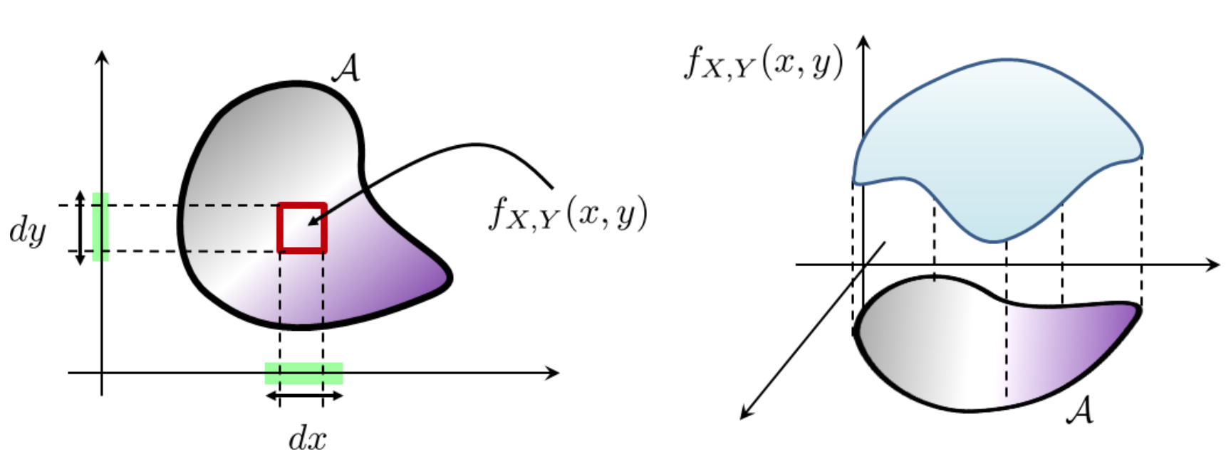
Fig. 9 A joint PDF for a pair of continuous random variables is a surface in the 2D plane. To measure the size of the event \(\eventA\), we integrate the surface function \(f_{X, Y}\) over the area covered by \(\eventA\). Image Credit: [Chan, 2021].

Normalization

Theorem 19 (Joint PMF and Joint PDF)

Let \(\S\) = \(\S_X \times \S_Y\). All joint PMFs and joint PDFs satisfy

(30)\[ \sum_{(x, y) \in \S} \pmfjointxy(x, y) = 1 \quad \text{and} \quad \int_{\S} \pdfjointxy(x, y) \, dx \, dy = 1 \]

Marginal PMF and PDF

To recover the PMF or PDF of a single random variable, we can marginalize the joint PMF or PDF by summing or integrating over the other random variable. More concretely, we define the marginal PMF and PDF below.

Definition 61 (Marginal PMF and PDF)

The marginal PMF is defined as

\[ p_X(x) = \sum_{y \in \S_Y} \pmfjointxy(x, y) \quad \text{and} \quad p_Y(y) = \sum_{x \in \S_X} \pmfjointxy(x, y) \]

and the marginal PDF is defined as

\[ f_X(x) = \int_{\S_Y} \pdfjointxy(x, y) \, dy \quad \text{and} \quad f_Y(y) = \int_{\S_X} \pdfjointxy(x, y) \, dx \]

Remark 10 (Marginal Distribution and the Law of Total Probability)

From Theorem 3, one can see that the definition of marginalization is closed related to the law of total probability. In fact, marginalization is a sum of conditioned observations.

In the chapter on Naive Bayes, we see that the denominator \(\mathbb{P}(\mathbf{X})\) can be derived by marginalization.

See the examples section in the chapter on Conditional PMF and PDF for a concrete example.

Example 12 (Marginal PDF of Bivariate Normal Distribution)

This example is adapted from [Chan, 2021].

A joint Gaussian random variable \((X, Y)\) has a joint PDF given by

\[ f_{X, Y}(x, y)=\frac{1}{2 \pi \sigma^2} \exp \left\{-\frac{\left(\left(x-\mu_X\right)^2+\left(y-\mu_Y\right)^2\right)}{2 \sigma^2}\right\} \]

The marginal PDFs \(f_X(x)\) and \(f_Y(y)\) are given by

\[\begin{split} \begin{aligned} f_X(x) & =\int_{-\infty}^{\infty} f_{X, Y}(x, y) d y \\ & =\int_{-\infty}^{\infty} \frac{1}{2 \pi \sigma^2} \exp \left\{-\frac{\left(\left(x-\mu_X\right)^2+\left(y-\mu_Y\right)^2\right)}{2 \sigma^2}\right\} d y \\ & =\frac{1}{\sqrt{2 \pi \sigma^2}} \exp \left\{-\frac{\left(x-\mu_X\right)^2}{2 \sigma^2}\right\} \cdot \int_{-\infty}^{\infty} \frac{1}{\sqrt{2 \pi \sigma^2}} \exp \left\{-\frac{\left(y-\mu_Y\right)^2}{2 \sigma^2}\right\} d y \end{aligned} \end{split}\]

Recognizing that the last integral is equal to unity because it integrates a Gaussian PDF over the real line, it follows that

\[ f_X(x)=\frac{1}{\sqrt{2 \pi \sigma^2}} \exp \left\{-\frac{\left(x-\mu_X\right)^2}{2 \sigma^2}\right\} \]

Similarly, we have

\[ f_Y(y)=\frac{1}{\sqrt{2 \pi \sigma^2}} \exp \left\{-\frac{\left(y-\mu_Y\right)^2}{2 \sigma^2}\right\} \]

Independence

In the case of bivariate random variables, independence means that the joint PMF or PDF can be factorized into the product of the PMF or PDF of the individual random variables. This is nothing but the definition of independence mentioned in chapter 2 (Definition 10).

More concretely, we define independence below.

Definition 62 (Independent random variables)

Random variables \(X\) and \(Y\) are independent if and only if

\[ \pmfjointxy(x, y) = p_X(x) p_Y(y) \quad \text{or} \quad \pdfjointxy(x, y) = f_X(x) f_Y(y) \]

Definition 63 (Independence for N random variables)

A sequence of random variables \(X_1\),…,\(X_N\) is independent if and only if their joint PDF (or joint PMF) can be factorized.

\[ f_{X_1, \ldots, X_n}(x_1, \ldots, x_n) = \prod_{n=1}^N f_{X_n}(x_n) \]

Independent and Identically Distributed (i.i.d.)

Definition 64 (Independent and Identically Distributed (i.i.d.))

Let \(X_1, X_2, \ldots, X_n\) be a sequence of random variables.

We say that the random variables are independent and identically distributed (i.i.d.) if the following two conditions hold:

1. The random variables are independent of each other. That is, \(P(X_i = x_i | X_j = x_j, j \neq i) = P(X_i = x_i)\) for all \(i, j\).

2. The random variables have the same distribution. That is, \(\P \lsq X_1 = x \rsq = \P \lsq X_2 = x \rsq = \ldots = \P \lsq X_n = x \rsq\) for all \(x\).

Corollary 10 (Joint PDF of \(\iid\) random variables)

An immediate consequence of the definition of \(\iid\) is that the joint PDF of \(\iid\) random variables can be written as a product of PDFs.

\[ f_{X_1, \ldots, X_n}(x_1, \ldots, x_n) = \prod_{n=1}^N f_{X_n}(x_n) \]

Remark 11 (Why is \(\iid\) so important?)

• If a set of random variables are \(\iid\), then the joint PDF can be written as a products of PDFs.

• Integrating a joint PDF is difficult. Integrating a product of PDFs is much easier.

The below two examples are taken from [Chan, 2021].

Example 13 (Gaussian \(\iid\))

Let \(X_1, X_2, \ldots, X_N\) be a sequence of \(\iid\) Gaussian random variables where each \(X_i\) has a PDF

\[ f_{X_i}(x) = \frac{1}{\sqrt{2 \pi}} \exp \lsq - \frac{x^2}{2} \rsq \]

The joint PDF of \(X_1, X_2, \ldots, X_N\) is

\[\begin{split} \begin{aligned} f_{X_1, \ldots, X_N}(x_1, \ldots, x_N) &= \prod_{i=1}^N \lsq \frac{1}{\sqrt{2 \pi}} \exp \lsq - \frac{x_i^2}{2} \rsq \rsq \\ &= (\frac{1}{\sqrt{2 \pi}})^N \exp \lsq - \sum_{i=1}^N \frac{x_i^2}{2} \rsq \\ \end{aligned} \end{split}\]

which is a function depending not on the individual values of \(x_1, x_2, \ldots, x_N\), but on the sum \(\sum_{i=1}^N x_i^2\). So we have “compressed” an N-dimensional function into a 1D function.

Example 14 (Gaussian \(\iid\) (cont.))

Let \(\theta\) be a deterministic number that was sent through a noisy channel. We model the noise as an additive \(\gaussian\) random variable with mean 0 and variance \(\sigma^2\). Supposing we have observed measurements \(X_i\) = \(\theta\) + \(W_i\), for i = 1, \(\ldots\) , N, where \(W_i\) ~ \(\gaussian\)(0, \(\sigma^2\)), then the PDF of each \(X_i\) is

\[ f_{X_i}(x) = \frac{1}{\sqrt{2 \pi \sigma^2}} \exp \lsq - \frac{(x - \theta)^2}{2 \sigma^2} \rsq \]

Thus the joint PDF of (\(X_1, X_2, \ldots, X_N\)) is

\[\begin{split} \begin{aligned} f_{X_1, \ldots, X_N}(x_1, \ldots, x_N) &= \prod_{i=1}^N \lsq \frac{1}{\sqrt{2 \pi \sigma^2}} \exp \lsq - \frac{(x_i - \theta)^2}{2 \sigma^2} \rsq \rsq \\ &= \lsq \frac{1}{\sqrt{2 \pi \sigma^2}} \rsq^N \exp \lsq - \sum_{i=1}^N \frac{(x_i - \theta)^2}{2 \sigma^2} \rsq \\ \end{aligned} \end{split}\]

Essentially, this joint PDF tells us the probability density of seeing sample data \(x_1, \ldots, x_N\).

Joint CDF

We now introduce the cumulative distribution function (CDF) for bivariate random variables. Similar to the 1-dimensional distribution, the joint CDF is a function that gives the probability in which both \(X\) and \(Y\) are less than or equal to some values \(x\) and \(y\), respectively.

The joint CDF is defined as follows.

Definition 65 (Joint CDF)

Let \(X\) and \(Y\) be two random variables. The joint CDF of \(X\) and \(Y\) is the function \(F_{X, Y}(x, y)\) such that

\[ F_{X, Y}(x, y)=\mathbb{P}[X \leq x \cap Y \leq y] \]

Definition 66 (Joint CDF (cont.))

If \(X\) and \(Y\) are discrete, then

\[ F_{X, Y}(x, y)=\sum_{y^{\prime} \leq y} \sum_{x^{\prime} \leq x} p_{X, Y}\left(x^{\prime}, y^{\prime}\right) \]

If \(X\) and \(Y\) are continuous, then

\[ F_{X, Y}(x, y)=\int_{-\infty}^y \int_{-\infty}^x f_{X, Y}\left(x^{\prime}, y^{\prime}\right) d x^{\prime} d y^{\prime} \]

If the two random variables are independent, then we have

\[ F_{X, Y}(x, y)=\int_{-\infty}^x f_X\left(x^{\prime}\right) d x^{\prime} \int_{-\infty}^y f_Y\left(y^{\prime}\right) d y^{\prime}=F_X(x) F_Y(y) \]