Cumulative Distribution Function
Contents
Cumulative Distribution Function#
The PMF is one way to describe the distribution of a discrete random variable. As we will see later on, PMF cannot be defined for continuous random variables. The cumulative distribution function (CDF) of a random variable is another method to describe the distribution of random variables. The advantage of the CDF is that it can be defined for any kind of random variable (discrete, continuous, and mixed) [Pishro-Nik, 2014].
The take away lesson here is that CDF is another way to describe the distribution of a random variable. In particular, in continuous random variables, we do not have an equivalent of PMF, so we use CDF instead.
Definition#
Definition 20 (Cumulative Distribution Function)
Let \(X\) be a discrete random variable with \(\S = \lset \xi_1, \xi_2, \ldots \rset\) where \(\xi_i \in \R\) for all \(i\). Note that \(X(\xi_i) = x_i\) for all \(i\) where \(x_i\) is the state of \(X\).
Then the cumulative distribution function \(\cdf\) is defined as
Since \(\P \lsq X = x_{\ell} \rsq\) is the probability mass function, we can also replace the symbol with the \(\pmf\) symbol.
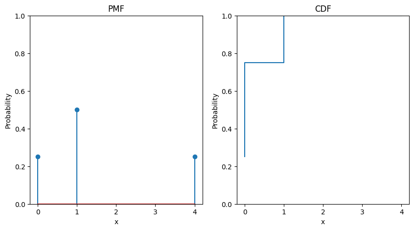
Example 8 (CDF)
Consider a random variable \(X\) with the following probability mass function:
Then by definition Definition 20, we have the CDF of \(X\) to be computed as:
Thus, our CDF is given by:
 1import warnings
 2
 3warnings.filterwarnings("ignore")
 4import numpy as np
 5import matplotlib.pyplot as plt
 6
 7p = np.array([0.25, 0.5, 0.25])
 8x = np.array([0, 1, 4])
 9F = np.cumsum(p)
10# plot 2 diagrams in one figure
11# y axis start from 0 to 1
12fig, ax = plt.subplots(1, 2, sharex=False, sharey=False, figsize=(10, 5))
13ax[0].set_ylim(0, 1)
14ax[0].set_title("PMF")
15ax[0].set_ylabel("Probability")
16ax[0].set_xlabel("x")
17ax[0].stem(x, p, use_line_collection=True)
18ax[0].grid(False)
19ax[1].set_ylim(0, 1)
20ax[1].set_title("CDF")
21ax[1].set_ylabel("Probability")
22ax[1].set_xlabel("x")
23ax[1].step(x, F)
24ax[1].grid(False)
25plt.show()
Properties#
Theorem 5 (Properties of CDF)
Let \(X\) be a discrete random variable with \(\S = \lset \xi_1, \xi_2, \ldots \rset\) where \(\xi_i \in \R\) for all \(i\). Then, the CDF \(\cdf\) of \(X\) satisfies the following properties:
The CDF is a staircase function and is non-decreasing. That is, for any \(\xi \in \S\), we have
\[ \cdf(x) \leq \cdf(x+1) \]The CDF is a probability function.
\[ 0 \leq \cdf(x) \leq 1 \]In particular, we have the minimum of the CDF is 0 and the maximum is 1 for \(x = -\infty\) and \(x = \infty\) respectively.
The CDF is right continuous.
PMF and CDF Conversion#
Theorem 6 (PMF and CDF Conversion)
Let \(X\) be a discrete random variable with \(\S = \lset \xi_1, \xi_2, \ldots \rset\) where \(\xi_i \in \R\) for all \(i\). Note that \(X(\xi_i) = x_i\) for all \(i\) where \(x_i\) is the state of \(X\). Then, the PMF of \(X\) can be obtained from the CDF by
where \(X\) has a countable set of states \(\S\).