Baye’s Theorem and the Law of Total Probability

Baye’s Theorem

Definition 13 (Baye’s Theorem)

Let \(\P\) be a probability function defined over the probability space \(\pspace\).

Two events \(A, B \in \E\) such that \(\P(A) > 0\) and \(\P(B) > 0\), we have

\[ \P(A|B) = \dfrac{\P(B|A)\P(A)}{\P(B)} \]

Proof. The observant reader should find it easy that this formula is deduced due to the fact that \(\P(A \cap B) = \P(B \cap A)\), and therefore

\[ \P(A|B) = \dfrac{\P(A\cap B)}{\P(B)} = \dfrac{\P(B \cap A)}{\P(B)} = \dfrac{\P(B ~|~ A)\P(A)}{\P(B)} \]

since \(\P(B ~|~ A) = \dfrac{\P(B \cap A)}{\P(A)}\).

Terminology (Posterior and Conditional Probability)

From the proof of Baye’s Theorem, we see that there are two ways to view \(\P(A \cap B)\). If the context is clear, we may call \(\P(B|A)\) the conditional probability and \(\P(A|B)\) the posterior probability.

Law of Total Probability

Theorem 3 (Law of Total Probability)

Let \(\P\) be a probability function defined over the probability space \(\pspace\).

Let \(\{A_1, \ldots, A_n\}\) be a partition of the sample space \(\S\). This means that \(A_1, \ldots, A_n\) are disjoint and \(\S = A_1 \cup \cdots \cup A_n\). Then, for any \(B \subseteq \S\), we have

\[ \P(B) = \sum_{i=1}^{n} \P(B|A_i)\P(A_i) \]

Intuition and Interpretation (Law of Total Probability)

The law of total probability can be stated more intuitively as the sum of event \(B\) and each of the disjoint event \(A_i\). We have to first recognize that the image below makes sense, assumming that the whole sample space can be made up of 3 disjoint events \(A_1, A_2, A_3\), and we see that event \(B\) touches all of them (i.e. there are overlaps), then it is obvious from the figure that \(\P(B)\) is the sum of \(\P(B \cap A_i)\). Note that event \(B\) does not necessarily need to touch all \(A_i\), if it doesn’t, then \(\P(B \cap A_i) = 0\).

Now if this intuition is established, we just express \(\P(B \cap A_i) = \P(B|A_i)\P(A_i)\) by conditional probability and we recovered back the formula for the law of total probability.

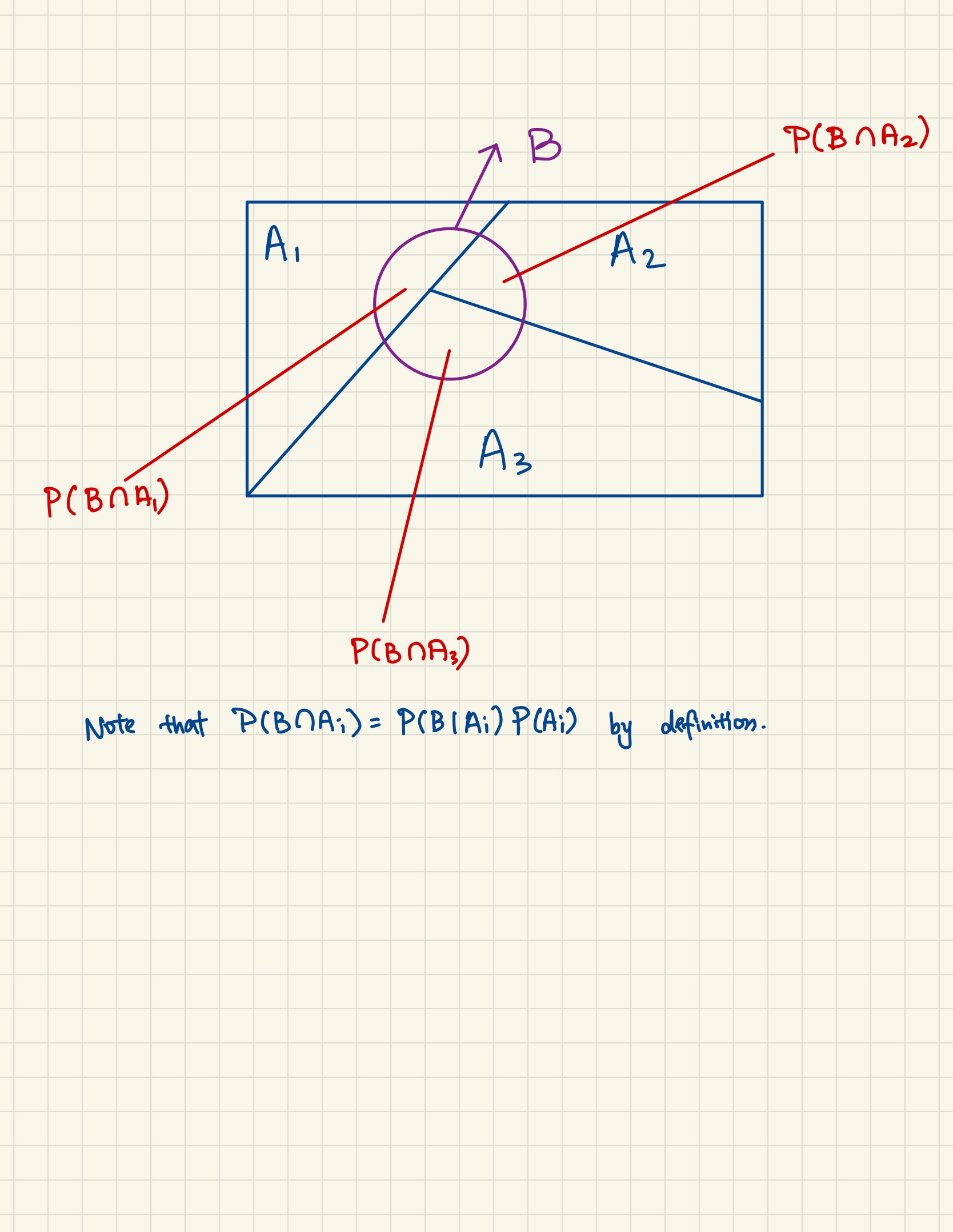
Fig. 4 Partition of Law of Total Probability.

The intuition of this is also apparent after understanding that if a sample space can be broken down into disjoint events \(A_1, A_2, \ldots, A_k\), then any event \(B\) that is in the sample space must touch some of these disjoint events, whenever they overlap, we can represent them as \(\P(A_i \cap B)\), and if we add them up it is just the event \(B\) itself. If they don’t overlap, we can still add them anyways since \(P(A_k \cap B) = 0\). Note the loose usage of the index here, \(i\) means overlap, \(k\) means non-overlap.

Corollary 6 (Law of Total Probability (Corollary))

Let \(\{A_1, \ldots, A_n\}\) be a partition of the sample space \(\S\). This means that \(A_1, \ldots, A_n\) are disjoint and \(\S = A_1 \cup \cdots \cup A_n\). Then, for any \(B \subseteq \S\), we have

\[ \P(A_j|B) = \dfrac{\P(B|A_j)\P(A_j)}{\sum_{i=1}^{n}\P(B|A_i)\P(A_i)} \]

Exercise 2.47 {#exercise-247}

Stanley H. Chan: Introduction to Probability for Data Science, 2021. (pp. 90-91)

Exercise 2.48 {#exercise-248}

Stanley H. Chan: Introduction to Probability for Data Science, 2021. (pp. 91)