K-Nearest Neighbours Decision Boundary

import numpy as np
import matplotlib.pyplot as plt
from sklearn import datasets, neighbors
# https://anaconda.org/conda-forge/mlxtend
from mlxtend.plotting import plot_decision_regions
import pandas as pd
from typing import List

def knn_comparision(data: pd.DataFrame, k: int) -> None:
    X = data[['x1','x2']].values
    y = data['y'].astype(int).values
    clf = neighbors.KNeighborsClassifier(n_neighbors=k)
    clf.fit(X, y)

    # Plotting decision regions
    plot_decision_regions(X, y, clf=clf, legend=2)

    # Adding axes annotations
    plt.xlabel('X1')
    plt.ylabel('X2')
    plt.title('Knn with K='+ str(k))
    plt.show()
    
def plot_knn_subplots(data_func, k_values: List[int]) -> None:
    """
    Plots k-NN decision regions for different k values using subplots.

    Parameters
    ----------
    data_func : callable
        Function to generate the data.
    k_values : List[int]
        List of k values for k-NN.
    """
    data = data_func()
    rows = int(np.ceil(len(k_values) / 3))
    fig, axes = plt.subplots(rows, 3, figsize=(15, 5 * rows))
    axes = axes.flatten()

    for idx, k in enumerate(k_values):
        X = data[["x1", "x2"]].values
        y = data["y"].astype(int).values
        clf = neighbors.KNeighborsClassifier(n_neighbors=k)
        clf.fit(X, y)

        # Plotting decision regions
        ax = axes[idx]
        plot_decision_regions(X, y, clf=clf, legend=2, ax=ax)

        # Adding axes annotations
        ax.set_xlabel("X1")
        ax.set_ylabel("X2")
        ax.set_title("Knn with K=" + str(k))

    plt.tight_layout()
    plt.show()

Overlapping Data

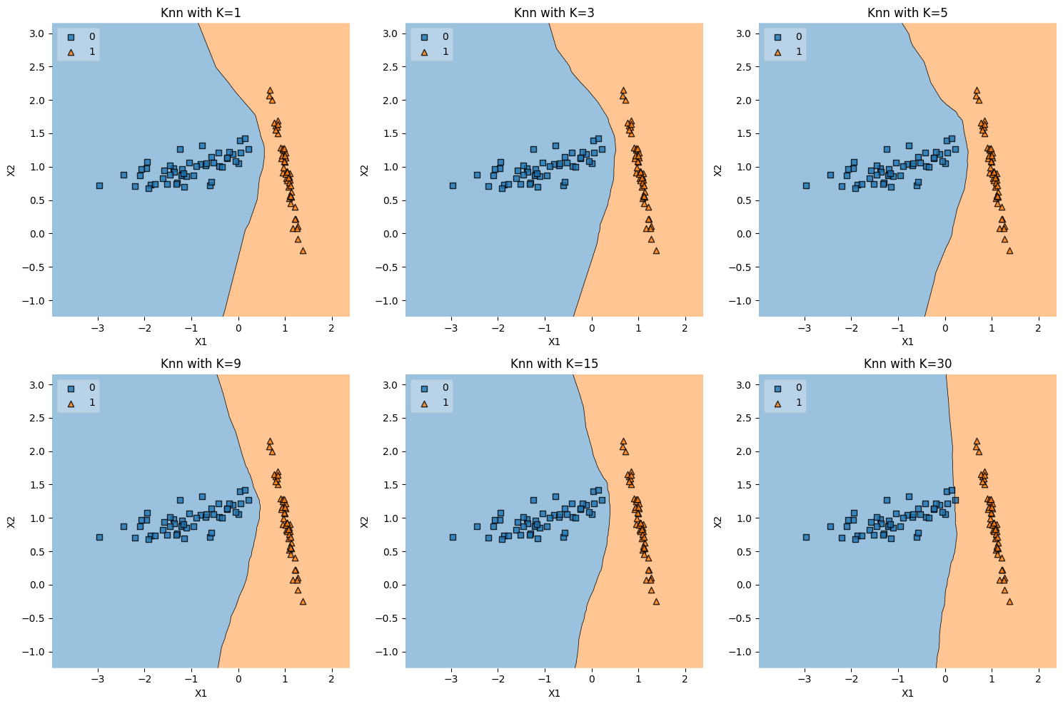
The term “overlapping data” typically refers to a situation where the data points belonging to different classes or categories are not well-separated and instead intermingle or overlap in the feature space. In the context of classification problems, overlapping data can make the task of learning a decision boundary more challenging.

The function overlapping_data() you provided is using the make_classification function from scikit-learn to generate a synthetic dataset with two features and two classes. The parameters n_features=2, n_redundant=0, and n_clusters_per_class=1 are controlling the characteristics of the generated data:

• n_features=2: Specifies that there are two features, so the data is 2-dimensional.

• n_redundant=0: Ensures that there are no redundant features, meaning that both features contribute information to the classification task.

• n_clusters_per_class=1: Specifies that there is only one cluster per class.

The combination of these parameters is likely to produce a dataset where the classes are not perfectly separated and may overlap to some extent. This makes the dataset useful for testing and visualizing classification algorithms, especially those that can handle non-linear decision boundaries, such as K-NN.

In summary, “overlapping data” in this context means that the data points from different classes are not clearly separated from each other, and there may be regions in the feature space where points from different classes are mixed together.

def overlapping_data() -> pd.DataFrame:
    X, y = datasets.make_classification(
        n_features=2, n_redundant=0, n_clusters_per_class=1
    )
    df = pd.DataFrame(dict(x1=X[:, 0], x2=X[:, 1], y=y))
    return df

k_values = [1, 3, 5, 9, 15, 30]
plot_knn_subplots(overlapping_data, k_values)

Ushape Data

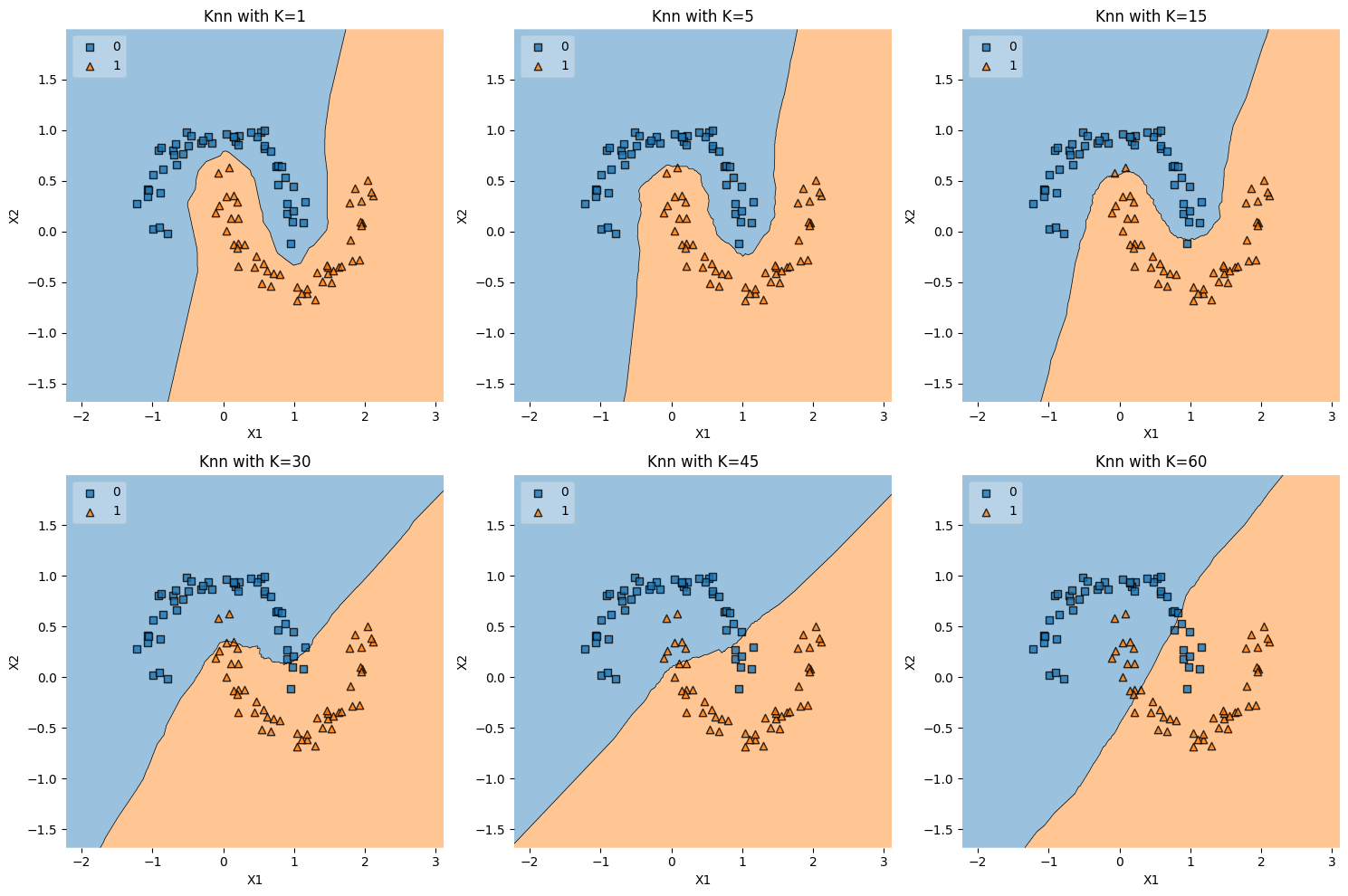
The function ushape_data() generates a dataset that consists of two “U”-shaped or crescent-shaped clusters. This is achieved using the datasets.make_moons function from scikit-learn, which is designed to create a binary classification dataset with two interleaving half-circles or “moons.” The parameter noise=0.1 adds some random noise to the data, making the separation between the classes less perfect.

Here’s why U-shaped data (or moon-shaped data) is interesting and often used:

1. Non-Linear Separation

The two classes in U-shaped data cannot be perfectly separated by a linear decision boundary. This makes the dataset a useful test case for evaluating classifiers that can handle non-linear decision boundaries, such as k-NN, decision trees, and kernel SVM.

2. Visualization

The U-shaped pattern is visually distinct and easy to recognize. When visualizing the decision boundaries of different classifiers, the U-shaped data helps in illustrating how various algorithms capture or fail to capture the non-linear patterns in the data.

3. Benchmarking

Because the underlying pattern of U-shaped data is well-understood, it can be used as a benchmark to compare the performance of different algorithms on a non-trivial, non-linear classification task.

4. Overfitting Demonstration

The U-shaped pattern can be sensitive to noise and the choice of hyperparameters. This sensitivity makes it a good dataset for demonstrating concepts like overfitting and the importance of hyperparameter tuning.

5. Clustering Analysis

Beyond classification, the U-shaped data can also be used to evaluate clustering algorithms, particularly those designed to detect non-convex clusters.

Conclusion

U-shaped data is a standard synthetic dataset used in machine learning to demonstrate, test, and compare algorithms capable of non-linear classification or clustering. It provides a clear and intuitive example of a situation where linear models are insufficient, thus showcasing the strengths and weaknesses of various algorithms in handling complex patterns.

def ushape_data() -> pd.DataFrame:
    X, y = datasets.make_moons(noise=0.1)
    df = pd.DataFrame(dict(x1=X[:,0], x2=X[:,1], y=y))
    return df

k_values = [1, 5, 15, 30, 45, 60]
plot_knn_subplots(ushape_data, k_values)

Linear Separability

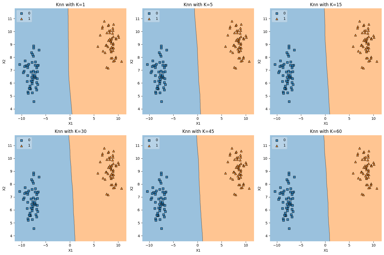
The function linear_sep_data() generates a dataset that consists of two linearly separable clusters or “blobs.” This is achieved using the datasets.make_blobs function from scikit-learn with parameters n_features=2 and centers=2, which creates two clusters in a two-dimensional feature space.

Here’s an explanation of what’s happening in the code and why this type of data is useful:

1. Creating Linearly Separable Data

• datasets.make_blobs is used to generate isotropic Gaussian blobs for clustering or classification tasks.

• n_features=2 specifies that there are two features, making the data 2-dimensional.

• centers=2 specifies that there are two distinct centers, leading to two well-separated clusters.

2. K-NN Classification

• The plot_knn_subplots function (defined earlier) is called with the linear_sep_data function and a list of \(K\) values.

• For each value of \(K\), a K-NN classifier is trained on the data, and the decision regions are plotted. Since the data is linearly separable, even a small value of \(K\) should be able to classify the data perfectly or near-perfectly.

3. Visualizing Decision Boundaries

• The subplots show how the decision boundary of the K-NN algorithm changes with different values of \(K\).

• You might observe that the decision boundary becomes smoother as \(K\) increases, reflecting the increased regularization effect of considering more neighbors.

4. Interest in Linearly Separable Data

• Linearly separable data is useful for demonstrating algorithms that can find a linear decision boundary, such as linear SVM or logistic regression.

• It can also be used to show how more complex models like K-NN or non-linear SVM can adapt to linear as well as non-linear patterns.

• It serves as a simple baseline case to understand the behavior of different algorithms.

Conclusion

The code snippet generates a dataset with two linearly separable clusters and then applies K-NN classification for different values of \(K\), visualizing the decision regions in subplots. This helps in understanding how the K-NN algorithm behaves on a simple dataset where the classes can be perfectly separated by a straight line, and how the choice of \(K\) affects the decision boundary. It’s a valuable tool for illustrating fundamental concepts in classification and model complexity.

def linear_sep_data() -> pd.DataFrame:
    X, y = datasets.make_blobs(n_features=2, centers=2)
    df = pd.DataFrame(dict(x1=X[:,0], x2=X[:,1], y=y))
    return df

k_values = [1, 5, 15, 30, 45, 60]
plot_knn_subplots(linear_sep_data, k_values)

XOR Data

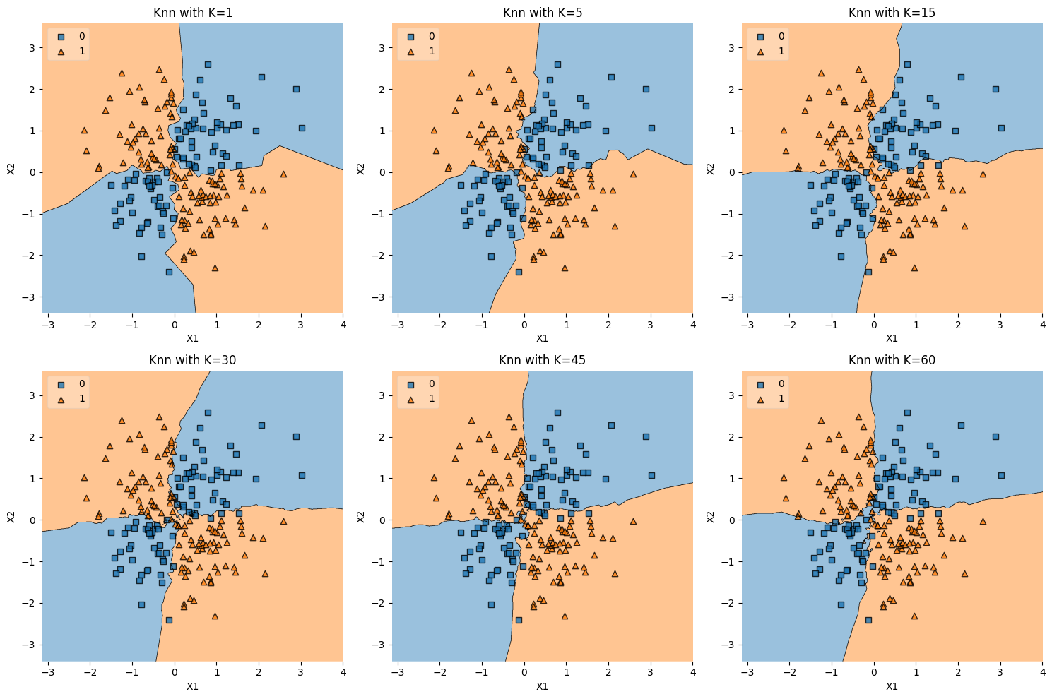
The xor_data() function generates a synthetic dataset that represents the XOR (exclusive or) problem, and then you’re using k-NN to classify this data for various values of \(K\).

XOR Data

The XOR function returns true if exactly one of its inputs is true, and false otherwise. In the context of a 2-dimensional feature space, the XOR problem can be visualized as having two classes where:

• Class 1: Points in the first and third quadrants.

• Class 2: Points in the second and fourth quadrants.

Here’s an explanation of the code:

1. Generating Data:

   • X = np.random.randn(200, 2): Creates 200 random data points in a 2-dimensional space, drawn from a standard normal distribution.

   • y = np.logical_xor(X[:, 0] > 0, X[:, 1] > 0): Computes the XOR operation on the signs of the two features for each data point, effectively dividing the space into the XOR pattern.

2. K-NN Classification:

   • The plot_knn_subplots function is called with the xor_data function and a list of \(K\) values.

   • For each value of \(K\), a k-NN classifier is trained on the XOR data, and the decision regions are plotted.

3. Visualizing Decision Boundaries:

   • The subplots show how the decision boundary of the k-NN algorithm changes with different values of \(K\).

   • The XOR problem is inherently non-linear, and the decision boundary will reflect the complex shape of the XOR pattern.

Interest in XOR Data

• Non-Linearity: The XOR problem is a classic example of a problem that is not linearly separable. No straight line can perfectly separate the classes.

• Benchmarking: XOR is often used to test the ability of algorithms to capture non-linear patterns.

• Understanding Model Complexity: Different values of \(K\) will show how the complexity of the model affects the ability to capture the XOR pattern. Smaller values of \(K\) may capture the pattern more closely but may also overfit to noise, while larger values of \(K\) may generalize better but fail to capture the pattern precisely.

Conclusion

The code snippet generates a dataset representing the XOR problem and applies k-NN classification for different values of \(K\), visualizing the decision regions in subplots. It serves as an illustrative example of a non-linear classification problem and demonstrates how k-NN can adapt to complex decision boundaries, depending on the choice of \(K\). It’s a valuable example for studying the behavior of non-linear classifiers and understanding the trade-offs between fitting complexity and generalization.

def xor_data() -> pd.DataFrame:
    X = np.random.randn(200, 2)
    y = np.logical_xor(X[:, 0] > 0, X[:, 1] > 0)
    df = pd.DataFrame(dict(x1=X[:,0], x2=X[:,1], y=y.astype(int)))
    return df

k_values = [1, 5, 15, 30, 45, 60]
plot_knn_subplots(xor_data, k_values)

Two Spirals Data

The two-spirals dataset is a visually compelling and mathematically complex pattern that has been a significant benchmark problem in machine learning. Here’s why it’s interesting and the rationale behind its use:

1. Complexity and Non-Linearity

• Pattern: The two-spirals dataset consists of points arranged in two intertwined spirals. This creates a non-linear and intricate boundary between the two classes.

• Challenge: There is no straight line that can separate the two classes, making it a non-trivial problem for machine learning algorithms.

2. Historical Significance in Neural Networks

• Early Benchmark: The two-spirals problem was used as a benchmark problem to test early neural networks.

• Understanding Hidden Layers: It helped researchers understand the importance of hidden layers and non-linear activation functions in capturing complex patterns.

3. Testing Non-Linear Algorithms

• Robust Test: The problem serves as a robust test for algorithms capable of handling non-linear decision boundaries, such as k-NN, SVM with non-linear kernels, and deep learning models.

• Hyperparameter Tuning: It’s valuable for tuning hyperparameters, such as the number of neighbors in k-NN.

4. Visualization and Interpretation

• Visual Appeal: The two-spirals problem provides a visually appealing way to illustrate the behavior of different algorithms.

• Understanding Overfitting: The complex pattern can lead to overfitting if the model is too flexible. It’s an excellent case to study the trade-offs between model complexity and generalization.

5. Rationale Behind Two Spirals Code

• Generation: The code generates two spirals by taking the square root of random numbers, scaling them, and applying sine and cosine functions. Noise can be added to make the pattern less perfect.

• Negative Mirror: One spiral is generated, and its negative mirror image forms the second spiral (X1 and X2 in the code).

• Binary Classification: The dataset is constructed for a binary classification task, where each spiral represents one class.

Conclusion

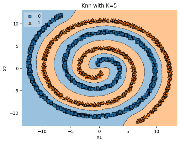
The two-spirals problem is not just visually intriguing but also carries rich historical and practical significance in the field of machine learning. It’s a benchmark for understanding non-linear decision boundaries, the capabilities of different algorithms, overfitting, and the role of hyperparameters. The generated dataset offers a tangible way to explore and visualize these critical concepts. By using the k-NN algorithm with \(K = 5\), as in your example, you can see how this specific model captures the complex boundary between the spirals, shedding light on its ability to handle non-linear patterns.

def two_spirals_data(n_points: int, noise: float = 0.5) -> pd.DataFrame:
    n = np.sqrt(np.random.rand(n_points, 1)) * 780 * (2 * np.pi) / 360
    d1x = -np.cos(n) * n + np.random.rand(n_points, 1) * noise
    d1y = np.sin(n) * n + np.random.rand(n_points, 1) * noise
    X1 = np.hstack((d1x, d1y))
    X2 = np.hstack((-d1x, -d1y))
    X = np.vstack((X1, X2))
    y = np.hstack((np.zeros(n_points), np.ones(n_points)))
    df = pd.DataFrame(dict(x1=X[:, 0], x2=X[:, 1], y=y.astype(int)))
    return df

knn_comparision(two_spirals_data(1000), 5)

S-Curve Data

def s_curve_data() -> pd.DataFrame:
    X, y = datasets.make_s_curve(n_samples=1000)
    df = pd.DataFrame(dict(x1=X[:,0], x2=X[:,2], y=y > 0))
    return df

k_values = [1, 5, 15, 30, 45, 60]
plot_knn_subplots(s_curve_data, k_values)

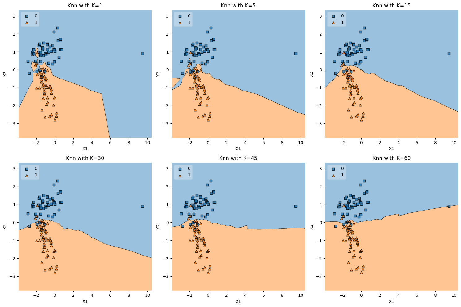
Outlier Data

Explanation

• Generation: The outlier_data() function creates a two-class, two-feature dataset using make_classification. Then, an outlier is manually introduced by shifting one data point far from the others (X[0][0] += 10).

• Effect of Outlier: By adding an outlier, the distribution of the data is skewed, potentially affecting the decision boundary.

• k-NN Classification: Different values of \(K\) are used to show how the decision boundary changes in the presence of an outlier.

Why is Outlier Data Interesting?

• Sensitivity to Outliers: Some models, especially when using small values of \(K\) in k-NN, are highly sensitive to outliers. This dataset helps in understanding and visualizing that sensitivity.

• Robustness Testing: By observing how different values of \(K\) handle the outlier, we can gain insights into the robustness of the model.

• Real-World Scenarios: Outliers are common in real-world data, so understanding their effect on different algorithms is essential.

Conclusion

Outlier Data helps in understanding the sensitivity and robustness of models to outliers, reflecting real-world data challenges.

def outlier_data() -> pd.DataFrame:
    X, y = datasets.make_classification(
        n_features=2, n_redundant=0, n_clusters_per_class=1
    )
    X[0][0] += 10  # Adding an outlier
    df = pd.DataFrame(dict(x1=X[:, 0], x2=X[:, 1], y=y))
    return df

k_values = [1, 5, 15, 30, 45, 60]
plot_knn_subplots(outlier_data, k_values)

Concetric Circles Data

Explanation

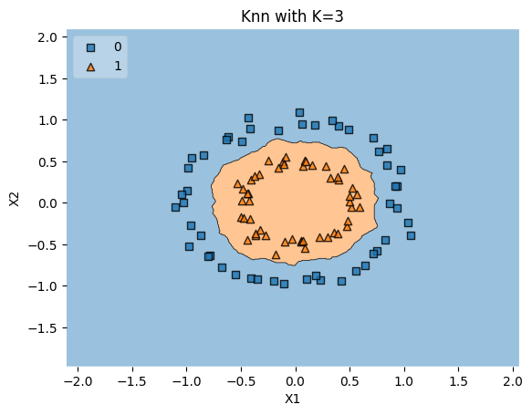
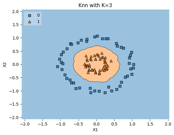
• Generation: The concentric_circles_data() function creates two classes arranged in concentric circles using datasets.make_circles. The factor parameter controls the distance between the circles.

• Non-Linearity: This dataset is not linearly separable, as the classes form concentric patterns.

• k-NN Classification: The k-NN algorithm is applied to classify the data with \(k=3\), using two different values of the factor to show how changing the distance between the circles affects classification.

Why is Concentric Circles Data Interesting?

• Complex Decision Boundaries: The concentric pattern requires a complex decision boundary, providing a robust test for algorithms capable of non-linear classification.

• Understanding Model Flexibility: By changing the factor, you can observe how the model adapts to different levels of complexity in the pattern.

• Benchmarking Non-Linear Models: Like the XOR and two-spirals problems, the concentric circles dataset is another classic benchmark for testing non-linear classifiers.

Conclusion

Concentric Circles Data serves as a test for non-linear classifiers and provides insights into model flexibility and complexity.

def concentric_circles_data(factor=0.5) -> pd.DataFrame:
    X, y = datasets.make_circles(noise=0.05, factor=factor)
    df = pd.DataFrame(dict(x1=X[:,0], x2=X[:,1], y=y))
    return df

knn_comparision(concentric_circles_data(factor=0.5), k=3)
knn_comparision(concentric_circles_data(factor=0.3), k=3)