Implementation

Implementation#

Training curve for amount of data#

from typing import Callable, Tuple

import matplotlib.pyplot as plt
import numpy as np
from sklearn.datasets import load_digits
from sklearn.metrics import accuracy_score
from sklearn.model_selection import train_test_split
from sklearn.svm import SVC


def generate_data() -> Tuple[np.ndarray, np.ndarray]:
    """Generate synthetic data for binary classification."""
    X, y = load_digits(return_X_y=True)
    return X, y


def learning_curve(
    estimator: Callable,
    scorer: Callable,
    X: np.ndarray,
    y: np.ndarray,
    start: int = 100,
    step: int = 100,
    n_runs: int = 5,
) -> Tuple[np.ndarray, np.ndarray, np.ndarray, np.ndarray]:
    """Compute the learning curve for a Support Vector Classifier model."""
    train_scores_runs = []
    val_scores_runs = []

    for _ in range(n_runs):
        seed = np.random.randint(0, 1000)
        X_train, X_val, y_train, y_val = train_test_split(
            X, y, test_size=0.2, random_state=seed
        )

        train_sizes = np.arange(start, len(X_train) + 1, step)

        train_scores = []
        val_scores = []

        for m in range(start, len(X_train) + 1, step):
            estimator.fit(X_train[:m], y_train[:m])

            train_score = scorer(y_train[:m], estimator.predict(X_train[:m]))
            val_score = scorer(y_val, estimator.predict(X_val))

            train_scores.append(train_score)
            val_scores.append(val_score)

        train_scores_runs.append(train_scores)
        val_scores_runs.append(val_scores)

    train_mean = np.mean(train_scores_runs, axis=0)  # mean of acc column
    val_mean = np.mean(val_scores_runs, axis=0)  # mean of acc column
    train_std = np.std(train_scores_runs, axis=0)
    val_std = np.std(val_scores_runs, axis=0)

    return train_sizes, train_mean, val_mean, train_std, val_std


def plot_learning_curve(
    train_sizes: np.ndarray,
    train_mean: np.ndarray,
    val_mean: np.ndarray,
    train_std: np.ndarray,
    val_std: np.ndarray,
    start: int = 100,
    step: int = 100,
) -> None:
    """Plot the learning curve with standard deviation fill."""
    x_values = np.arange(start, len(train_mean) * step + start, step)
    np.testing.assert_array_equal(x_values, train_sizes)

    plt.plot(x_values, train_mean, "r-+", linewidth=2, label="Training set")
    plt.fill_between(
        x_values,
        train_mean - train_std,
        train_mean + train_std,
        alpha=0.1,
        color="r",
    )

    plt.plot(x_values, val_mean, "b-s", linewidth=3, label="Validation set")
    plt.fill_between(
        x_values,
        val_mean - val_std,
        val_mean + val_std,
        alpha=0.1,
        color="b",
    )

    plt.xlabel("Training set size")
    plt.ylabel("Accuracy")
    plt.legend(loc="lower right")
    plt.title("Learning curve")
    plt.show()


# Generate synthetic data
X, y = generate_data()

# Initialize the model
model = SVC(kernel="rbf", gamma=0.001)
scorer = accuracy_score

# Compute learning curve
train_sizes, train_mean, val_mean, train_std, val_std = learning_curve(
    model, accuracy_score, X, y, start=100, step=100, n_runs=5
)
print(train_sizes, train_mean, val_mean, train_std, val_std)

# Plot learning curve with standard deviation fill
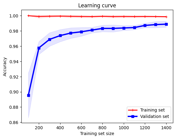
plot_learning_curve(train_sizes, train_mean, val_mean, train_std, val_std)

[ 100  200  300  400  500  600  700  800  900 1000 1100 1200 1300 1400] [1.         0.999      0.99933333 0.9995     0.9992     0.999
99885714 0.99925    0.99888889 0.999      0.99890909 0.999
99892308 0.99871429] [0.89555556 0.95777778 0.96888889 0.97388889 0.97722222 0.97888889
98111111 0.98333333 0.98333333 0.98388889 0.98444444 0.98722222
98833333 0.98888889] [0.         0.002      0.00133333 0.001      0.0016     0.00133333
00106904 0.001      0.00140546 0.00126491 0.00106017 0.00097183
00061538 0.00069985] [0.02937623 0.00849837 0.0088541  0.00797372 0.00689426 0.00571979
00368514 0.00430331 0.00464811 0.00323942 0.00283279 0.00283279
00408248 0.00392837]

../../../_images/79ffab14394dcf7c8fafd8bd2c1befc817605c468ec7cfcd4299ceda5124865b.png

What this algorithm above is doing is the following:

We intend to use different seeds for more robust results. So we will run the experiment multiple times.
In each experiment, we will split the data into a training set and a validation set.
Then we define a start and step to indicate how many data points we want to use for training in the first iteration, and how many data points we want to add in each iteration.
- For example, if start is \(100\) and step is \(100\), then we will use \(100\) data points for training in the first iteration, and \(200\) data points for training in the second iteration, and so on.
Assume we have \(1000\) data points in total.
- Training set: \(900\) data points
- Validation set: \(100\) data points
Assume start is \(100\) and step is \(100\).
- Iteration 1: \(100\) data points for training, producing hypothesis \(h_1\), and use \(h_1\) to evaluate the loss function on the training set and the validation set. Note that the validation set is the same for all iterations, to be \(100\) data points.
- Iteration 2: \(200\) data points for training, producing hypothesis \(h_2\), and use \(h_2\) to evaluate the loss function on the training set and the validation set. Note that the validation set is the same for all iterations, to be \(100\) data points.
- Iteration 3: \(300\) data points for training, producing hypothesis \(h_3\), and use \(h_3\) to evaluate the loss function on the training set and the validation set. Note that the validation set is the same for all iterations, to be \(100\) data points.
- …
- Iteration 9: \(900\) data points for training, producing hypothesis \(h_9\), and use \(h_9\) to evaluate the loss function on the training set and the validation set. Note that the validation set is the same for all iterations, to be \(100\) data points.
So we now have \(9\) hypotheses, \(h_1, h_2, \ldots, h_9\), and \(9\) training losses, train_loss_1, train_loss_2, …, train_loss_9, and \(9\) validation losses, val_loss_1, val_loss_2, …, val_loss_9. We can now plot the training loss and the validation loss as a function of the number of training examples.
An additional layer of complexity is that we want to run the experiment multiple times, say \(3\) times, and we want to plot the average training loss and the average validation loss as a function of the number of training examples.
Everything is the same, just that we compile the training loss and the validation loss for each iteration for each experiment, and then we average them. Represented as a matrix below, we see:

\[\begin{split} \text{train_loss} = \begin{bmatrix} \text{train_loss_11} & \text{train_loss_12} & \cdots & \text{train_loss_19} \\ \text{train_loss_21} & \text{train_loss_22} & \cdots & \text{train_loss_29} \\ \text{train_loss_31} & \text{train_loss_32} & \cdots & \text{train_loss_39} \\ \end{bmatrix} \end{split}\]

\[\begin{split} \text{val_loss} = \begin{bmatrix} \text{val_loss_11} & \text{val_loss_12} & \cdots & \text{val_loss_19} \\ \text{val_loss_21} & \text{val_loss_22} & \cdots & \text{val_loss_29} \\ \text{val_loss_31} & \text{val_loss_32} & \cdots & \text{val_loss_39} \\ \end{bmatrix} \end{split}\]

where the matrix has \(3\) rows and \(9\) columns, each row representing the training loss and the validation loss for one experiment.

So we sum each column, and divide by \(3\) to get the average training loss and the average validation loss across the \(3\) experiments.

Training curve for number of iterations#

This is quite simple, we just need to plot the training loss and validation loss as a function of the number of iterations, especially in gradient based optimization algorithms (i.e. neural networks).

Implementation

Contents

Implementation#

Training curve for amount of data#

Training curve for number of iterations#