Concept#
Using Seed Number 1992
Intuition#
This section is adapted from Machine Learning, The Basics, by Alexander Jung[Jung, 2023]. Nearest Neighbor (NN) methods, including \(K\)-NN methods, are distinctive machine learning (ML) algorithms that construct a specific form of hypothesis space. They find application across various learning tasks such as regression (with numeric labels, e.g., \(\mathcal{Y} = \mathbb{R}\)) and classification (with categorical labels, e.g., \(\mathcal{Y} = \{-1, 1\}\)).
Metric Space Requirement#
NN methods mandate that the feature space \(\mathcal{X}\) be a metric space, where a metric defines the distance between distinct feature vectors.
For example, when the feature space is the Euclidean space \(\mathbb{R}^n\), the metric is given by the Euclidean distance
between two vectors \(\mathbf{x}, \mathbf{x}^{\prime} \in \mathbb{R}^n\).
Training and Hypothesis Space#
Given a training set \(\mathcal{S} = \left\{\left(\mathbf{x}^{(i)}, y^{(i)}\right)\right\}_{i=1}^m\), containing labeled data points, NN methods construct a hypothesis space of piece-wise constant functions
The function value \(h(\mathbf{x})\) for any hypothesis \(h\) in this space is determined solely by the \(K\) nearest neighbors in \(\mathcal{S}\) with respect to \(\mathbf{x}\). Here, \(K\) is a hyper-parameter, leading to the term \(K\)-NN methods.
Binary Classification Illustration#
To illustrate, let’s consider a binary classification task where \(K\) is an odd number (e.g., \(k = 3\) or \(k = 5\)). The aim is to predict the binary label \(y \in \{-1,1\}\) based on a feature vector \(\mathbf{x} \in \mathbb{R}^n\), utilizing a training set \(\mathcal{S}\) with \(m > k\) labeled data points.
For a given feature vector \(\mathbf{x}\), let \(\mathcal{N}^{(k)}\) represent a set of \(K\) data points from \(\mathcal{S}\) having the smallest distance to \(\mathbf{x}\). If we denote \(m_1^{(k)}\) and \(m_{-1}^{(k)}\) as the count of data points in \(\mathcal{N}^{(k)}\) with labels 1 and -1 respectively, the \(K\)-NN method “learns” a hypothesis \(\widehat{h}\):
Notable Characteristics#
Dependence on Training Set: The hypothesis space of \(K\)-NN relies on \(\mathcal{S}\), requiring access and storage of the training set to compute predictions \(h(\mathbf{x})\), leading to significant memory demands.
No Parameter Tuning: Unlike linear regression or deep learning, \(K\)-NN does not require the solution of optimization problems for model parameters, aside from choosing \(K\).
Conceptual Appeal: With low computational requirements (aside from memory), NN methods are conceptually appealing as natural approximations of Bayes estimators.
In summary, NN methods, including \(K\)-NN, are versatile, conceptually straightforward, yet require specific structural conditions on the feature space. Their simplicity and lack of need for parameter tuning contrasts with other ML methods, though they may raise issues related to storage requirements and potential sensitivity to the data.
Since the models keep the training examples around at test time, we call them exemplar-based models. (This approach is also called instance-based learning, or memory-based learning)[Murphy, 2022].
Problem Formulation for K-Nearest Neighbors (KNN)#
Given a set \(\mathcal{S}\) containing \(N\) data points:
where
\(\mathcal{X} = \mathbb{R}^D\) is the feature space,
\(\mathcal{Y} = \mathbb{R}\) for regression or \(\mathcal{Y} = \{0, 1, \dots, C-1\}\) for classification is the label space,
\(\mathbf{x}^{(n)}\) is the \(n\)-th sample with \(D\) number of features,
\(y^{(n)}\) is its corresponding label.
Here both \(\mathbf{x}^{(n)}\) and \(y^{(n)}\) are drawn from an unknown joint distribution \(\mathcal{D}\).
The K-Nearest Neighbors algorithm is a non-parametric method that classifies an unlabeled instance \(\mathbf{x}^{(q)}\) based on the majority vote of its \(K\) nearest labeled neighbors in the training set if it is a classification problem, or predicts its label as the average of the labels of its \(K\) nearest neighbors if it is a regression problem.
The Nearest Neighbour Set and the Distance Metric#
Define \(\mathcal{N}_K(\mathbf{x}^{(q)}, d(\cdot), \mathcal{S})\) to be the set of \(K\) nearest neighbors of \(\mathbf{x}^{(q)}\) in the training set \(\mathcal{S}\), according to the distance metric \(d\):
where
\(d(\cdot)\) is a distance metric that measures the similarity between two data points.
\(d^{(n')} = d\left(\mathbf{x}^{n'}, \mathbf{x}^{(q)}\right)\) is the distance between \(\mathbf{x}^{(n')}\) and \(\mathbf{x}^{(q)}\).
The set includes the \(y^{(n)}\) labels of the \(K\) nearest neighbors of \(\mathbf{x}^{(q)}\) in the training set \(\mathcal{S}\) for convenience. In actual fact, we only need the \(K\) nearest neighbors of \(\mathbf{x}^{(q)}\) with respect to the distance metric \(d(\cdot)\) on all the training samples \(\mathbf{x}^{(n)}\) and do not depend on the labels \(y^{(n)}\).
The most commonly used distance metric is the Euclidean distance:
However, other distance metrics such as the Manhattan distance and the cosine distance can also be used.
Probabilistic Interpretation of K-Nearest Neighbors#
Given a new input \(\mathbf{x}^{(q)}\), the KNN classifier aims to find the \(K\) closest examples to \(\mathbf{x}^{(q)}\) in the training set, denoted \(\mathcal{N}_K(\mathbf{x}^{(q)}, d(\cdot), \mathcal{S})\), and then derive a distribution over the labels for the local region around \(\mathbf{x}\). More precisely, we compute:
where
\(c = 0, 1, \dots, C-1\) is a class label in the label space \(\mathcal{Y}\),
\(\mathbb{I}(\cdot)\) is the indicator function that returns \(1\) if the condition is true and \(0\) otherwise.
We can then return this distribution or the majority label.
Classification#
The K-Nearest Neighbors algorithm for classification defines a function \(\mathcal{F}(\cdot)\) that maps an unlabeled instance \(\mathbf{x}^{(q)}\) to a label in \(\mathcal{Y}\):
or more explicitly:
Here, \(\mathcal{S}\) denotes the training set, and \(d(\cdot)\) denotes the distance metric used to determine the nearest neighbors.
In short, we do the following:
Given one query point \(\mathbf{x}^{(q)}\) from the test set \(\mathcal{S}_{\text{test}}\), we aim to assign \(\mathbf{x}^{(q)}\) a label.
Calculate the distance from the test query point to all other points in the train dataset.
We sort and then store the \(K\) nearest neighbors (data points).
Get the majority class from these neighbors.
Return this class as the prediction.
This formalism can be related to the probabilistic interpretation by recognizing that the majority vote corresponds to selecting the class with the highest estimated probability:
Note that the probabilistic interpretation of KNN aligns with the non-parametric nature of the algorithm, estimating the conditional probability distribution over labels based on local similarities in the feature space \(\mathcal{X}\). It also provides a connection to the underlying distribution of the data \(\mathcal{D} = \mathbb{P}_{\mathcal{D}}\), as it assumes that the labels are drawn according to this distribution within the local region around \(\mathbf{x}^{(q)}\).
Regression#
For regression, the K-Nearest Neighbors algorithm defines a function \(\mathcal{F}(\cdot)\) that maps an unlabeled instance \(\mathbf{x}^{(q)}\) to a real value in \(\mathcal{Y}\):
In short, we do the following:
Calculate the distance from the test query point $\mathbf{x}^{(q)} to all other points in the train dataset.
We sort and then store the \(K\) nearest neighbors (data points).
Get the majority class from these neighbors.
Take the mean of the top \(K\) nearest labels and return the mean as the prediction.
Summary#
The goal of the K-Nearest Neighbors algorithm, whether for classification or regression, is to predict the labels of unlabeled instances in a manner that is consistent with the underlying distribution of the labels in the neighborhood of each instance. It assumes that instances close in the feature space are likely to have similar labels.
The algorithm has no explicit training phase but relies on the entire training set for prediction. Consequently, the complexity of the model grows linearly with the size of the training set, making it computationally expensive for large datasets. Moreover, the choice of \(K\) (the number of neighbors) and the distance metric can have a significant impact on the model’s performance. A small value of \(K\) may make the model sensitive to noise, while a large value may smooth out the decision boundaries too much.
KNN has been widely applied in various domains, including pattern recognition, anomaly detection, and recommendation systems. Its simplicity and flexibility to adapt to different types of data and problems make it a popular choice among practitioners. However, it may suffer from the curse of dimensionality and requires careful preprocessing and parameter tuning to perform optimally.
In summary, K-Nearest Neighbors provides an intuitive and straightforward way to perform classification (or regression) based on the principle that similar instances are likely to have similar outputs. Its non-parametric nature allows it to capture complex relationships without relying on a specific functional form, but it requires careful consideration of the hyperparameters and the underlying assumptions about the data.
Our Focus (K-Nearest Neighbors Classification)#
We will primarily focus on the K-Nearest Neighbors algorithm for classification in this chapter.
K-Nearest Neighbors Convergence#
Murphy wrote in his book the following:
The K-Nearest Neighbors (KNN) classifier becomes within a factor of 2 of the Bayes error as \(N \to \infty\)[Murphy, 2022].
For a more concrete proof, see CS4780.
Here’s why I think is the case:
1. Convergence of Nearest Neighbors#
As the number of data points \(N\) approaches infinity, the nearest neighbors of a given query point will converge to the true underlying distribution of the data. This means that the local regions around the query point will become increasingly representative of the global distribution.
2. Density Estimation#
KNN effectively acts as a non-parametric density estimator. By considering the majority vote of the \(K\) nearest neighbors, KNN estimates the conditional probability \(P(Y = y | \mathbf{x})\) for a given query point \(\mathbf{x}\). As \(N \to \infty\), this estimate converges to the true conditional probability, assuming the conditions for consistency are met (such as choosing \(K\) to grow with \(N\) but at a slower rate).
3. Bayes Classifier#
The Bayes classifier is the optimal classifier that assigns a label to a query point based on the true conditional probability \(P(Y = y | \mathbf{x})\). The Bayes error is the lowest possible error that can be achieved by any classifier, and it represents the inherent noise or overlap in the data distribution.
4. KNN Convergence to Bayes Classifier#
As \(N \to \infty\), the KNN estimate of the conditional probability converges to the true conditional probability, and thus the KNN decision rule approaches the Bayes decision rule. The error rate of the KNN classifier approaches the Bayes error.
5. Factor of 2 Result#
The specific result that the error rate of the KNN classifier is at most twice the Bayes error rate can be proven rigorously using mathematical analysis. It relies on the assumptions that the data is drawn independently from a stationary distribution and that certain conditions on \(K\) and \(N\) are met.
In summary, the convergence of the KNN error rate to within a factor of 2 of the Bayes error is a manifestation of the algorithm’s statistical consistency and its ability to approximate the true underlying distribution of the data as the sample size grows. It’s a powerful result that illustrates the theoretical strength of KNN despite its simplicity. It also underscores the importance of the choice of \(K\) and the distance metric, as well as the assumptions about the underlying data distribution, in achieving this convergence.
Hypothesis Space for K-Nearest Neighbors (KNN)#
The hypothesis space \(\mathcal{H}\) for KNN encompasses all possible functions that can be defined by considering the \(K\) nearest neighbors for classification.
Definition for Classification#
Given a set of \(N\) labeled data points \(\left\{\left(\mathbf{x}^{(n)}, y^{(n)}\right)\right\}_{n=1}^N\), where \(y^{(n)} \in \mathcal{Y}\) (e.g., \(\mathcal{Y} = \{0, 1, \dots, C-1\}\) for a \(C\)-class classification problem), the class of functions \(\mathcal{H}\) for KNN can be written as:
Here:
\(\mathcal{X} = \mathbb{R}^D\) is the feature space.
\(\mathcal{Y}\) is the set of possible labels (e.g., \(\mathcal{Y} = \{0, 1, \dots, C-1\}\) for a \(C\)-class classification problem).
\(\mathcal{N}_K\left(\mathbf{x}^{(q)}, d(\cdot), \mathcal{S}\right)\) denotes the set of \(K\) nearest neighbors of \(\mathbf{x}\) in the training set.
\(\mathbb{I}(\cdot)\) is the indicator function.
This definition represents the class of functions that can be constructed using the KNN algorithm, considering different choices of \(K\), distance metrics, and training data.
General Definition and Properties#
The hypothesis space \(\mathcal{H}\) in KNN consists of all possible functions that map a query point \(\mathbf{x}\) to a label \(y\), based on the \(k\) nearest neighbors in the training set \(\mathcal{S}\). Given a specific value of \(k\) and distance function \(d\), the hypothesis space can be formally defined as:
Summary#
Unlike K-Means, where the hypothesis space has finite cardinality, the hypothesis space for KNN is more complex and depends on the continuous nature of the feature space and the choice of \(K\). It reflects the non-parametric nature of KNN, where the algorithm’s flexibility allows it to capture complex relationships in the data without relying on a specific functional form.
In summary, the hypothesis space for KNN encapsulates the algorithm’s ability to classify data points based on local similarities and the principle that similar instances in the feature space are likely to have similar labels. Its richness and complexity mirror the inherent flexibility and adaptability of the KNN algorithm.
Loss, Cost and Objective Functions???#
The K-Nearest Neighbors (KNN) algorithm is a non-parametric method, meaning it doesn’t learn parameters from the training data through optimization. Instead, it relies on the entire training set to make predictions. Because of this, there is no specific cost, loss, or objective function that needs to be minimized during a training phase.
See this post in stackexchange for more info.
If you really want, there is no stopping you from defining a loss function for KNN to check for “goodness” of the model. But, it is not necessary.
Loss Function: The empirical risk can be defined using various loss functions \(\mathcal{L}\), such as the 0-1 loss for classification or mean squared error for regression:
\[ \hat{\mathcal{R}}_{\mathcal{S}}(h_{\mathcal{S}, K}) = \frac{1}{N} \sum_{n=1}^{N} \mathcal{L}\left( y^{(n)}, h_{\mathcal{S}, k}(\mathbf{x}^{(n)}) \right) \]Generalization: The performance of KNN on new data points can be studied through statistical learning theory. The true risk under the data-generating distribution \(\mathcal{D}\) can be expressed as:
\[ \mathcal{R}_{\mathcal{D}}(h_{\mathcal{S}, K}) = \mathbb{E}_{(\mathbf{x}, y) \sim \mathcal{D}}\left[ \mathcal{L}\left( y, h_{\mathcal{S}, K}(\mathbf{x}) \right) \right] \]
Algorithm#
Remark 5 (Choice of K and Distance Metric)
The choice of \(K\) and the distance metric can have a significant impact on the performance of the KNN algorithm. A small value of \(K\) may make the algorithm sensitive to noise, while a large value may lead to over-smoothing. Cross-validation can be used to select an appropriate value of \(K\). Similarly, the choice of distance metric should be appropriate for the nature of the data (e.g., Euclidean for continuous features, Hamming for binary features).
Algorithm 3 (K-Nearest Neighbors (KNN) Algorithm)
Given a set of labeled data points (training samples)
and a new unlabeled instance \(\mathbf{x}^{(q)}\), the KNN algorithm aims to predict the label of \(\mathbf{x}\) based on the \(K\) closest examples in \(\mathcal{S}\).
Choose the Number of Neighbors (K): Select a value for \(K\), which is the number of nearest neighbors to consider for classification.
Compute Distances: Calculate the distance between \(\mathbf{x}\) and each data point in \(\mathcal{S}\). The distance metric (e.g., Euclidean distance) can be chosen based on the problem domain.
\[ \begin{aligned} d^{(n)}\left(\mathbf{x}^{(q)}, \mathbf{x}^{(n)}\right) = \left\| \mathbf{x}^{(q)} - \mathbf{x}^{(n)} \right\|^2 \end{aligned} \]Select K Nearest Neighbors: Identify the \(K\) data points in \(\mathcal{S}\) with the smallest distances to \(\mathbf{x}^{(q)}\). This set of nearest neighbors is denoted as \(\mathcal{N}_K(\mathbf{x}^{(q)})\).
\[\begin{split} \begin{aligned} \mathcal{N}_K\left(\mathbf{x}^{(q)}, d(\cdot), \mathcal{S}\right) &= \left\{\left(\mathbf{x}^{(n)}, y^{(n)}\right) \mid n \in \text{argmin}_i^K d\left(\mathbf{x}^{(i)}, \mathbf{x}^{(q)}\right) \right\} \\ &= \left\{ \left(\mathbf{x}^{(n)}, y^{(n)}\right) \mid n \in \underset{n'}{\operatorname{argmin}} \left\{ d^{(n')}\right\}, n' = 1, 2, \ldots, K \right\} \end{aligned} \end{split}\]Compute the Predicted Label: Determine the predicted label for \(\mathbf{x}^{(q)}\) based on the labels of its \(K\) nearest neighbors. For classification, this can be done by taking a majority vote among the nearest neighbors.
\[ \begin{aligned} \hat{y} = \arg\max_{y \in \mathcal{Y}} \sum_{\left(\mathbf{x}^{(n)}, y^{(n)}\right) \in \mathcal{N}_K\left(\mathbf{x}^{(q)}, d(\cdot), \mathcal{S}\right)} \mathbb{I}\left(y^{(n)} = y\right) \end{aligned} \]where \(\mathbb{I}(\cdot)\) is the indicator function.
The predicted label \(\hat{y}\) represents the classification of the new instance \(\mathbf{x}^{(q)} based on its \)K$ nearest neighbors in the training set.
This algorithm represents the standard operation of KNN for classification. If used for regression, step 4 would involve computing a mean or weighted mean of the target values of the \(K\) nearest neighbors instead of a majority vote.
Time Complexity of Naive (Brute-Force) KNN#
Euclidean Distance Calculation: The time complexity for calculating the Euclidean distance between two points of dimension \(\mathbb{R}^D\) is \(\mathcal{O}(D)\), as it involves \(D\) subtractions, \(D\) squares, and \((D-1)\) additions with one square root operation at the end.
Distance Computation for All Training Examples:
For each test sample, calculating the distance to all \(N\) training examples takes \(\mathcal{O}(N \cdot D)\).
Sorting the Distances:
Sorting the distances for each test sample takes \(\mathcal{O}(N \cdot \log N)\).
Calculating Majority Class:
Determining the majority class based on the \(K\) nearest neighbors takes \(\mathcal{O}(K)\) time.
Total Time Complexity for a Single Query:
The overall complexity for one test sample is \(\mathcal{O}(N \cdot D + N \cdot \log N + K)\) but since \(K \ll N\), the time complexity is \(\mathcal{O}(N \cdot D + N \cdot \log N)\).
Total Time Complexity for Multiple Queries:
If there are \(P\) test samples, the final time complexity is \(\mathcal{O}(P \cdot N \cdot D + P \cdot N \cdot \log N)\).
Space Complexity of Naive (Brute-Force) KNN#
Input Matrix: The space required for the training data \(\mathcal{X}\) is \(\mathcal{O}(N \cdot D)\).
Distance List: The space required for storing the distances to all training examples (for a single query) is \(\mathcal{O}(N)\).
Total Space Complexity:
The overall space complexity is \(\mathcal{O}(N \cdot D + N)\), which simplifies to \(\mathcal{O}(N \cdot D)\) since \(N \cdot D\) is usually the dominant term.
Summary#
Time Complexity:
\(\mathcal{O}(P \cdot N \cdot D + P \cdot N \cdot \log N)\) for \(P\) test samples.
Space Complexity:
\(\mathcal{O}(N \cdot D)\).
The naive K-NN’s time complexity is primarily influenced by the number of training examples, the dimensionality of the feature space, and the number of test samples. The space complexity is determined by the size of the training data. This detailed analysis aligns with the practical implementation of the brute-force K-NN method, highlighting the computational challenges that may arise with large datasets or high-dimensional feature spaces.
Other K-NN Methods and Their Time and Space Complexity#
I will not go into the details of these methods, but I will provide a brief overview of their time and space complexity. The table below summarizes the complexity of the QuickSelect, Ball Tree, and KD-Tree methods.
Method |
Operation |
Best Case Time |
Average Case Time |
Worst Case Time |
Space Complexity |
Description |
|---|---|---|---|---|---|---|
QuickSelect |
Finding \(K\)-th smallest element |
\(\mathcal{O}(N)\) |
\(\mathcal{O}(N)\) |
\(\mathcal{O}(N^2)\) |
\(\mathcal{O}(1)\) |
QuickSelect is used to find the \(K\)-th smallest element, with average linear time but a worst-case quadratic time. |
Ball Tree |
Build |
\(\mathcal{O}(N \log N)\) |
\(\mathcal{O}(N \log N)\) |
\(\mathcal{O}(N \log N)\) |
\(\mathcal{O}(N)\) |
Building a Ball Tree involves partitioning data into hyper-spheres. |
Ball Tree |
Query |
\(\mathcal{O}(\log N)\) |
\(\mathcal{O}(\log N)\) |
\(\mathcal{O}(N)\) |
\(\mathcal{O}(N)\) |
Querying a Ball Tree is usually logarithmic but can degrade to linear time in the worst case. |
KD-Tree |
Build |
\(\mathcal{O}(N \log N)\) |
\(\mathcal{O}(N \log N)\) |
\(\mathcal{O}(N \log N)\) |
\(\mathcal{O}(N)\) |
Building a KD-Tree involves partitioning space along axes-aligned hyperplanes. |
KD-Tree |
Query |
\(\mathcal{O}(\log N)\) |
\(\mathcal{O}(\log N)\) |
\(\mathcal{O}(N)\) |
\(\mathcal{O}(N)\) |
Querying a KD-Tree is usually logarithmic but can degrade to linear time in the worst case. |
Example#
We illustrate the KNN classifier in \(2d\) in Fig. 12 for \(K=5\). The test point is marked as an \(\mathrm{x}\). 3 of the 5 nearest neighbors have label 1, and 2 of the 5 have label 0 . Hence we predict \(p(y=1 \mid \boldsymbol{x}, \mathcal{D})=3 / 5=0.6\)[Murphy, 2022].
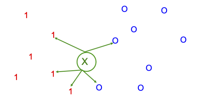
Fig. 12 Illustration of a \(K\)-nearest neighbors classifier in 2d for \(K=5\). The nearest neighbors of test point \(\boldsymbol{x}\) have labels \(\{1,1,1,0,0\}\), so we predict \(p(y=1 \mid \boldsymbol{x}, \mathcal{S})=3 / 5\). Image Credit: [Murphy, 2022].#
K-Nearest Neighbors (KNN) and Voronoi Regions#
The K-Nearest Neighbors classifier classifies an unlabeled instance \(\mathbf{x}^{(q)}\) based on the majority vote of its \(K\) nearest labeled neighbors in the training set. For the case of \(K = 1\), the decision boundaries can be visualized using Voronoi regions.
Voronoi Regions for 1-NN#
Given a training set \(\mathcal{S}\), the Voronoi region for a particular training example \(\left(\mathbf{x}^{(n)}, y^{(n)}\right)\) is defined as the set of all points that are closer to \(\mathbf{x}^{(n)}\) than to any other training example in \(\mathcal{S}\):
The Voronoi regions partition the feature space \(\mathbb{R}^D\) into disjoint cells, where each cell corresponds to one training example.
This definition says that the Voronoi region \(\mathcal{V}_n\) for the \(n\)-th training example consists of all points \(\mathbf{x}\) in the feature space that are closer to \(\mathbf{x}^{(n)}\) than to any other training example.
Characteristics of 1-NN Voronoi Regions#
When \(K = 1\) in the K-Nearest Neighbors (KNN) algorithm, several unique characteristics emerge:
Delta Function Predictive Distribution: The predicted label for a query point \(\mathbf{x}^{(q)}\) is exactly the label of its nearest neighbor, resulting in a delta function predictive distribution[Murphy, 2022].
Voronoi Tessellation: The Voronoi regions create a partitioning of the feature space, with each region corresponding to a training point.
Zero Training Error: The model will perfectly classify all training points, leading to zero training error.
Overfitting: A 1-NN model may overfit the training data and perform poorly on unseen data.
Classification Using Voronoi Regions#
Given an unlabeled instance \(\mathbf{x}^{(q)}\), and if \(K=1\), then the 1-NN algorithm assigns the label of the training example whose Voronoi region contains \(\mathbf{x}^{(q)}\):
Example#
Let’s illustrate with an example from Probablistic Machine Learning, An Introduction by Kevin Murphy[Murphy, 2022].
import numpy as np
import matplotlib.pyplot as plt

from scipy.spatial import KDTree, Voronoi, voronoi_plot_2d

np.random.seed(42)
data = np.random.rand(25, 2)
vor = Voronoi(data)

print("Using scipy.spatial.voronoi_plot_2d, wait...")
voronoi_plot_2d(vor)
xlim = plt.xlim()
ylim = plt.ylim()

plt.show()

print("Using scipy.spatial.KDTree, wait a few seconds...")
plt.figure()
tree = KDTree(data)
x = np.linspace(xlim[0], xlim[1], 200)
y = np.linspace(ylim[0], ylim[1], 200)
xx, yy = np.meshgrid(x, y)
xy = np.c_[xx.ravel(), yy.ravel()]
plt.plot(data[:, 0], data[:, 1], "ko")
plt.pcolormesh(x, y, tree.query(xy)[1].reshape(200, 200), cmap="jet")

plt.show()
Using scipy.spatial.voronoi_plot_2d, wait...

Using scipy.spatial.KDTree, wait a few seconds...

Extending to \(K > 1\)#
For \(K > 1\), the decision boundaries are more complex and cannot be described by simple Voronoi regions. However, the concept of local similarity still applies, and the algorithm classifies an unlabeled instance based on the majority vote of its \(K\) nearest neighbors.
Geometrical Structure of K-Nearest Neighbors (KNN) Hypothesis Space#
The KNN algorithm’s hypothesis space reveals a rich geometrical structure, defined through Voronoi tessellation. The space can be understood as the class of all functions that are piecewise constant on the cells of the \(K\)-th order Voronoi diagram of a given set of \(n\) points in \(\mathbb{R}^D\).
Voronoi Tessellation in KNN#
For a collection of training examples \(\{\mathbf{x}^{(n)}\}_{n=1}^N \subset \mathbb{R}^D\), let \(\mathcal{V}_j^K(\{\mathbf{x}^{(n)}\}_{n=1}^N)\) be the \(j\)-th Voronoi cell in the \(K\)-th order Voronoi partition of the space. This means that all the points in each of these cells have the same \(K\)-nearest neighbors among \(\{\mathbf{x}^{(n)}\}_{n=1}^N\). The class of functions underlying \(K\)-NN can be written as:
Connection to Previous Discussion#
This geometrical perspective connects to the earlier description of the KNN hypothesis space by emphasizing the piecewise constant nature of the KNN functions. It showcases how the Voronoi cells, defined by the training examples, form the underlying structure that drives the classification or regression decision.
The piecewise constant behavior in each Voronoi cell aligns with the KNN algorithm’s logic, where the prediction for a query point is determined by the majority label or average value among the \(K\)-nearest neighbors. This local decision-making process is manifested in the geometrical partitioning of the space into Voronoi cells, where each cell encapsulates the influence of the corresponding training examples.
The hypothesis space for KNN, through the lens of Voronoi tessellation, offers a profound understanding of the algorithm’s ability to adapt to local patterns in the data. This geometrical view complements the decision-making perspective, providing a comprehensive picture of the KNN algorithm’s richness, flexibility, and complexity. It illustrates how the choice of \(K\) and the spatial distribution of training examples shape the function space, allowing the KNN algorithm to capture intricate relationships in the feature space.
Summary#
In summary, the concept of Voronoi regions applies to the KNN algorithm for the special case of \(K = 1\), where it defines the decision boundaries for classification. The Voronoi regions partition the feature space into cells, each corresponding to a training example, and the algorithm assigns labels based on these regions. For larger values of \(K\), the decision boundaries are more complex, and the simple Voronoi partitioning no longer applies, but the underlying principle of local similarity remains the same.
However, when \(k=1\) the KNN algorithm creates a highly flexible model that adapts perfectly to the training data but may lack robustness and generalization to new, unseen data. This setting captures the idiosyncrasies of the training data at the cost of potentially poor performance on data not included in the training set. The Voronoi tessellation provides a geometric interpretation of this behavior, visualizing the decision boundaries formed by the nearest neighbors.
The Curse of Dimensionality in K-Nearest Neighbors (K-NN)#
The effectiveness of the K-NN algorithm relies on the notion that similar points in the feature space likely share similar labels. This assumption, however, breaks down in high-dimensional spaces due to the phenomenon known as the “curse of dimensionality.” In high-dimensional spaces, points drawn from a probability distribution tend to be far apart, making the concept of closeness or similarity less meaningful.
Illustration Using Hyper-Cube#
A unit hypercube is a geometric shape in \(D\)-dimensional space where all sides have a length of 1. It’s the generalization of a square in two dimensions and a cube in three dimensions to \(D\) dimensions.
In mathematical terms, the unit hypercube in \(\mathbb{R}^D\) can be defined as:
Here, \([0,1]\) refers to the closed interval from 0 to 1, and \([0,1]^D\) means that each of the \(D\) dimensions of the hypercube ranges from 0 to 1. All the edges are parallel to the axes, and all angles between edges are right angles.
Consider the unit hyper-cube \(\mathcal{C} = [0,1]^D\) in \(D\)-dimensional space. Suppose all training data points \(\left\{\mathbf{x}^{(n)}\right\}_{n=1}^N\) are sampled uniformly within this cube, and we are interested in the \(K=10\) nearest neighbors of a test point \(\mathbf{x}^{(q)}\) within \(\mathcal{C}\).
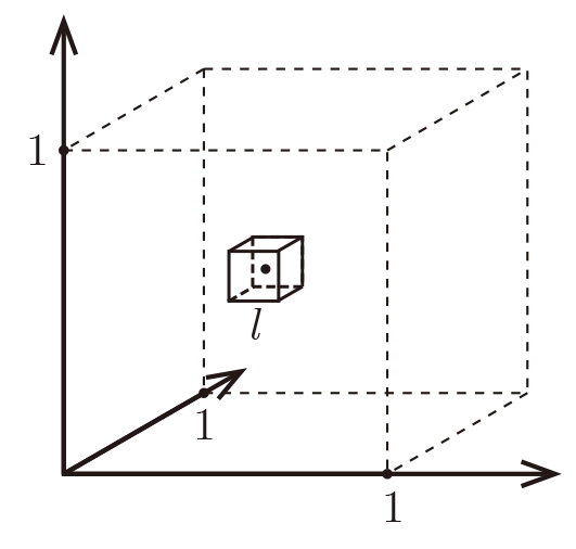
Let \(\ell\) be the edge length of the smallest hyper-cube that contains all \(K\)-nearest neighbors of \(\mathbf{x}^{(q)}\). Then the volume of this hyper-cube is \(\ell^D\), and we can approximate:
Given \(K=10\) and \(N=1000\), the following table shows how \(\ell\) grows with the dimension \(D\):
Dimension (\(D\)) |
Length (\(\ell\)) |
|---|---|
2 |
0.1 |
10 |
0.63 |
100 |
0.955 |
1000 |
0.9954 |
Implications#
As \(D\) grows significantly large, almost the entire space is needed to find the \(K\)-NN. This breakdown of the K-NN assumptions occurs because the \(K\)-nearest neighbors are not particularly closer to \(\mathbf{x}^{(q)}\) than any other data points in the training set. The notion of similarity, and consequently the rationale for sharing labels, becomes ambiguous.
In other words, given a test point \(\mathbf{x}^{(q)}\), and if dimension \(D\) is large, then the \(K\)-nearest neighbors of \(\mathbf{x}^{(q)}\) are not significantly closer to \(\mathbf{x}^{(q)}\) than any other data points in the training set.
Required Number of Data Points#
One might think of increasing the number of training samples, \(N\), to make the nearest neighbors truly close to the test point. However, the required number of samples grows exponentially with the dimension. To achieve \(\ell = \frac{1}{10} = 0.1\), we would need:
For dimensions greater than 100, this would require more data points than there are electrons in the universe.
Conclusion#
The curse of dimensionality presents a significant challenge for the K-NN algorithm in high-dimensional spaces. It undermines the foundational assumption of similarity and requires an impractical number of samples for effective learning. This phenomenon emphasizes the importance of dimensionality reduction and careful feature selection when applying K-NN to real-world high-dimensional problems.
See Curse of Dimensionality for more details.
Decision Boundary#
Definition of Decision Boundary#
The decision boundary in K-NN is a hypersurface that partitions the feature space \(\mathcal{X} = \mathbb{R}^D\) into regions corresponding to different classes. Given a distance metric \(d(\cdot)\), the number of neighbors \(K\), and a training set \(\mathcal{S}\), the decision boundary is defined as the locus of points \(\mathbf{x}^{(q)}\) in \(\mathcal{X}\) where there is a tie in the majority vote among the \(K\) nearest neighbors, or equivalently, where the estimated class probabilities are equal.
Mathematical Description#
Given the training set
and the label space \(\mathcal{Y} = \{0, 1, \dots, C-1\}\), the decision boundary for a specific pair of classes \(c_1\) and \(c_2\) is defined as the set of points \(\mathbf{x}^{(q)}\) for which
where
and \(N_K(\mathbf{x}^{(q)}, d(\cdot), \mathcal{S})\) is the set of \(K\) nearest neighbors of \(\mathbf{x}^{(q)}\).
Properties of the Decision Boundary#
Complexity: The decision boundary can be highly complex or smooth, depending on the choice of \(K\). A small \(K\) leads to a complex, jagged boundary that may capture noise (potentially overfitting), while a large \(K\) leads to a smoother boundary that may oversimplify the underlying patterns.
Sensitivity to Noise: The decision boundary is sensitive to noise and outliers, especially for small \(K\). Misclassified training examples near the boundary can distort it.
Non-Linearity: The decision boundary in K-NN is not restricted to be linear. It can adapt to the underlying distribution of the data, capturing non-linear relationships.
Local Decision Making: The decision boundary is determined by local information, specifically the \(K\) nearest neighbors. This reflects the instance-based nature of K-NN, where decisions are made based on localized regions of the feature space.
Influence of Distance Metric: The shape and position of the decision boundary are influenced by the chosen distance metric \(d(\cdot)\). Different metrics may lead to different boundaries.
In summary, the decision boundary in K-NN is a fundamental concept that describes how the algorithm classifies instances in the feature space. Its properties are influenced by the choice of hyperparameters, the nature of the data, and the underlying assumptions of the algorithm. Understanding the decision boundary helps in interpreting the behavior of K-NN and in tuning its parameters for optimal performance.
Mathematical Description for \(C\) Classes#
Given the same training set and label space as before, the decision boundaries for \(C\) classes are defined by the set of points in the feature space where the estimated class probabilities are tied for at least two classes. Mathematically, the decision boundary is the set of points \(\mathbf{x}^{(q)}\) that satisfy:
where the class probability is defined as before:
Properties and Characteristics#
Multiple Boundaries: For \(C\) classes, there will be multiple decision boundaries separating the regions corresponding to different classes.
Higher Complexity: The geometry of the decision boundaries becomes more complex as the number of classes increases, especially if the classes are not well-separated.
Intersecting Boundaries: Decision boundaries for different pairs of classes may intersect, creating a network of hypersurfaces that partitions the feature space.
Local Decision Making: The decision boundaries are still determined by local information, specifically the \(K\) nearest neighbors. The local structure of the data dictates how the boundaries are formed.
Non-Linearity: As with the binary case, the decision boundaries in K-NN are not restricted to being linear. They can capture complex, non-linear relationships between classes.
Visualization#
Visualizing the decision boundaries for more than two classes can be challenging, especially in high-dimensional spaces. In two dimensions, the decision boundaries can be visualized as lines (or curves) that separate the plane into regions corresponding to different classes. In three dimensions, the boundaries become surfaces, and in higher dimensions, they are hypersurfaces.
Summary#
The generalization of the decision boundary concept to \(C\) classes in K-NN follows the same principles as the binary case but with added complexity due to the increased number of classes. Understanding these decision boundaries can be valuable for interpreting the behavior of the algorithm, diagnosing potential issues, and fine-tuning the hyperparameters for optimal performance in multi-class classification tasks.
The decision boundary in a classification problem serves as a critical concept that separates the feature space into distinct regions corresponding to different classes. Intuitively, it’s like a frontier or a dividing line that helps the model decide which class a new observation belongs to based on its features. Let’s delve into why decision boundaries are useful and why having a tie on the boundary signifies something important.
Why Decision Boundaries Are Useful#
Understanding Classification Behavior: The decision boundary provides a visual and mathematical representation of how the algorithm classifies different regions of the feature space. It helps in understanding how changes in features affect the predicted class.
Identifying Class Boundaries: It demarcates where one class ends and another begins. This can be vital for understanding how well the model can distinguish between classes.
Analyzing Model Complexity: The shape and structure of the decision boundary can give insights into the complexity of the model. A linear boundary may suggest a simple relationship between features and classes, while a highly non-linear, jagged boundary might indicate overfitting.
Evaluating Sensitivity to Features: By examining the decision boundary, one can understand how sensitive the classification is to changes in different features. It helps in identifying which features have more influence on the classification.
Assessing Multi-Class Dynamics: In multi-class problems, decision boundaries show how classes relate to each other in the feature space, revealing potential challenges in distinguishing some classes from others.
Why a Tie on the Boundary Signifies Something#
A tie on the decision boundary means that the algorithm is equally uncertain about assigning an observation on the boundary to either of the adjacent classes. Here’s why it’s significant:
Critical Point of Decision Making: A tie signifies that the observation lies exactly on the point where the algorithm cannot favor one class over the other. It’s like standing right on the border between two countries.
Sensitivity to Noise and Model Parameters: Observations on or near the decision boundary may be highly sensitive to noise in the data or changes in model parameters (like the distance metric or \(K\) in K-NN). A small change might lead to a different classification.
Highlighting Ambiguities: Ties on the decision boundary highlight areas where the model may struggle to make clear distinctions between classes. It can reveal regions of ambiguity that might need special attention, such as gathering more features or tuning hyperparameters.
Guidance for Model Improvement: Understanding where and why ties occur on the decision boundary can guide further model development, including feature engineering, selection of distance metrics, or choice of \(K\) in K-NN.
Summary#
The decision boundary acts as a geographical map of how the classification algorithm interprets the feature space. Ties on this boundary reveal critical points where the model is most uncertain and sensitive. Understanding these aspects of the decision boundary can lead to a more intuitive grasp of the model’s behavior, better diagnostic insights, and guidance for model refinement and improvement.
Assumptions#
The K-Nearest Neighbors (K-NN) algorithm is relatively straightforward, but it operates under certain assumptions that can impact its performance. Here are the major assumptions:
1. Homogeneous Feature Scale#
The scale of the variables matters in K-NN. All features must be on a similar scale; otherwise, features with larger scales will unduly influence the distance metric. This emphasizes the need for normalization or standardization.
2. Relevance of Euclidean Distance#
The K-NN algorithm assumes that the Euclidean distance (or other chosen distance metrics) is a meaningful measure of similarity between instances. If this assumption does not hold, the algorithm may not perform well.
3. Equal Importance of Features#
Unless feature weighting is employed, K-NN treats all features as equally important in the similarity measure. If one or more irrelevant features are included in the model, the performance can be adversely affected.
4. Data Distribution and Density#
K-NN assumes that the local structure or density of the data is informative. This means that instances that are close to one another in the feature space are assumed to have similar outputs.
5. Smooth Decision Boundary#
The algorithm assumes that the decision boundary is smooth, especially for larger values of \(K\). A very small \(K\) can capture more noise and result in a more complex and jagged boundary, which may lead to overfitting.
6. Independence of Observations#
K-NN assumes that the observations are independent of one another. If there are dependencies between observations, the algorithm might produce biased predictions.
7. Non-parametric Nature#
K-NN is a non-parametric method, meaning that it makes no explicit assumptions about the functional form of the transformation from features to output. While this adds to its flexibility, it also means that the algorithm relies heavily on the data itself, rather than any underlying parameters.
8. Noisy Data Sensitivity#
K-NN is sensitive to noisy data. Outliers or mislabeled examples can significantly influence the decision boundary, especially for small values of \(K\).
9. Curse of Dimensionality#
K-NN suffers from the curse of dimensionality. As the number of dimensions (features) increases, the distance between samples in the feature space becomes less meaningful, and more data are required to make reliable predictions.
Balanced Class Distribution
In classification problems, K-NN assumes that the classes are relatively balanced. If one class significantly outnumbers the others, the majority class may dominate the voting process, leading to biased predictions. This can result in the algorithm consistently predicting the majority class, particularly when the value of \(K\) is not carefully chosen. In such imbalanced scenarios, techniques like oversampling the minority class, undersampling the majority class, or using a weighted voting scheme may be required to obtain more accurate and unbiased predictions.
Including this assumption completes the list, giving a comprehensive overview of the factors that can influence the performance of the K-NN algorithm.
From Wikipedia with modification: examples of a more frequent class tend to dominate the prediction of the new example, because they tend to be common among the \(K\) nearest neighbors due to their large number. This is intuitive, as if our dataset contains 1 million samples, and 99% of it are of one label, and say we use a neighbour \(K=11\), then it is relatively likely our 11 nearest neighbours have the dominant class. One way to overcome this problem is to weight the classification, taking into account the distance from the test point to each of its \(K\) nearest neighbors.
Conclusion#
The effectiveness of the K-NN algorithm relies on these assumptions. Violating these assumptions can lead to poor performance. Proper preprocessing, such as feature scaling and selection, along with careful choice of hyperparameters like \(K\) and the distance metric, can mitigate some of these issues and enhance the performance of the K-NN algorithm.
Summary#
Instance-Based Learning: KNN is an example of an instance-based learning algorithm. Rather than summarizing the training data into a compact model, it uses the entire training dataset to make predictions. The rationale is that similar input examples are likely to have similar output values.
Lazy Learning: KNN is often referred to as a “lazy learning” algorithm because it defers most of the computation until a query is made. When a query point \(\mathbf{x}^{(q)}\) is presented, the algorithm calculates the distance from \(\mathbf{x}^{(q)}\) to every example in \(\mathcal{S}\) to find the k-nearest neighbors and predict the output.
Non-Parametric: The algorithm does not assume any specific form for the underlying distribution that generates the data. It makes no parametric assumptions, and thus, the model complexity grows with the size of the data. The data itself serves as a representation of the underlying function.
Memory vs. Computation Trade-off: By storing the entire training dataset, KNN leverages memory to reduce computation during the learning phase. However, this leads to increased computational complexity during the prediction phase, where distances must be computed to all stored instances.
KNN for Classification and Regression: KNN can be employed for both classification and regression tasks.
Classification: It assigns the mode of the labels of the top \(K\) nearest neighbors.
Regression: It assigns the mean of the labels of the top \(K\) nearest neighbors.
Refer to the illustration named “classification_vs_regression” for a visual representation.
Nature of KNN:
Non-parametric: KNN does not make explicit assumptions about the functional form of the distribution of data. This allows it to capture complex relationships without relying on specific assumptions that might not hold.
Instance-based and Supervised: KNN memorizes the training instances and uses them for prediction, requiring supervision through labeled data.
Algorithm Breakdown: The detailed steps of the KNN algorithm can be found in the Algorithm section.
Computational Considerations: KNN requires scanning the entire training set for each query, making it computationally expensive. Various techniques, such as dimensionality reduction (e.g., PCA) or clustering, can alleviate this issue.
Bias and Variance Tradeoff:
Bias: High bias may cause underfitting due to erroneous assumptions.
Variance: High variance may lead to overfitting due to sensitivity to fluctuations in the training set.
Refer to the Wikipedia section on KNN for formal mathematical definitions.
Hyperparameters:
\(K\): The number of neighbors, the selection of which is discussed in the Decision Boundary and \(K\) section.
Distance Metric \(\mathcal{d}\): Defines the measure of similarity between data points.
Handling Large Datasets: Techniques like dimensionality reduction, random sampling, and regional clustering can reduce computational cost.
Handling Missing Values: Missing values can be imputed using the average or majority class of the closest \(K\) neighbors.
Notable Properties of KNN:
Data Dependency: More data generally implies better KNN, as it provides a richer representation of the underlying distribution.
Choice of \(K\): \(K\) is usually chosen as an odd number to avoid ties. Small \(K\) leads to a complex decision surface, while large \(K\) smooths the surface.
Edge Cases: Special cases for \(K = 1\) and \(K = m\) are explained in the Decision Boundary and \(K\) section.
Normalization: Feature scaling is essential since KNN relies on distance measures. See the Normalization section.
This summary encapsulates the essential aspects of the KNN algorithm, adhering to the notations and rigor established in previous sections. It serves as a concise and comprehensive review for those studying the algorithm, with references to more detailed explanations and visualizations.
References#
https://www.cs.cornell.edu/courses/cs4780/2018fa/lectures/lecturenote02_kNN.html
kevinzakka’s end-to-end KNN: Primarily based off this reference.