\[ \newcommand{\R}{\mathbb{R}} \newcommand{\P}{\mathbb{P}} \newcommand{\1}{\mathbb{1}} \newcommand{\Pobj}{\mathbb{P}(\text{obj})} \newcommand{\yhat}{\symbf{\hat{y}}} \newcommand{\xhat}{\symbf{\hat{x}}} \newcommand{\x}{\symbf{x}} \newcommand{\y}{\symbf{y}} \newcommand{\w}{\symbf{w}} \newcommand{\h}{\symbf{h}} \newcommand{\bs}{\textbf{bs}} \newcommand{\byolo}{\mathrm{b}_{\text{yolo}}} \newcommand{\bgrid}{\mathrm{b}_{\text{grid}}} \newcommand{\cc}{\mathrm{c}} \newcommand{\iou}{\textbf{IOU}_{\symbf{\hat{b}}}^{\symbf{b}}} \newcommand{\conf}{\textbf{conf}} \newcommand{\confhat}{\hat{\textbf{conf}}} \newcommand{\X}{\symbf{X}} \newcommand{\xx}{\mathrm{x}} \newcommand{\yy}{\mathrm{y}} \newcommand{\ww}{\mathrm{w}} \newcommand{\hh}{\mathrm{h}} \newcommand{\xxhat}{\hat{\mathrm{x}}} \newcommand{\yyhat}{\hat{\mathrm{y}}} \newcommand{\wwhat}{\hat{\mathrm{w}}} \newcommand{\hhhat}{\hat{\mathrm{h}}} \newcommand{\gx}{\mathrm{g_x}} \newcommand{\gy}{\mathrm{g_y}} \newcommand{\b}{\symbf{b}} \newcommand{\bhat}{\symbf{\hat{b}}} \newcommand{\p}{\symbf{p}} \newcommand{\phat}{\symbf{\hat{p}}} \newcommand{\y}{\symbf{y}} \newcommand{\L}{\mathcal{L}} \newcommand{\lsq}{\left[} \newcommand{\rsq}{\right]} \newcommand{\lpar}{\left(} \newcommand{\rpar}{\right)} \newcommand{\jmax}{j_{\max}} \newcommand{\obji}{\mathbb{1}_{i}^{\text{obj}}} \newcommand{\nobji}{\mathbb{1}_{i}^{\text{noobj}}} \DeclareMathOperator*{\argmax}{arg\,max} \newcommand{\abs}{\text{abs}} \]

YOLOv1#

YOLO (You Only Look Once) is a single-stage object detector that frames object detection as a single regression problem to predict bounding box coordinates and class probabilities of objects in an image. The model is called YOLO because you only look once at an image to predict what objects are present and where they are in the image. There are several versions of YOLO models, with each one having a slightly different architecture from the others. In this article, we will focus on the very first model called YOLOv1.

YOLOv1 comprises of a single convolutional neural network that simultaneously predicts multiple bounding boxes and class probabilities for these boxes. Compared to other traditional methods of object detection such as DPM and R-CNN, the YOLO model has several benefits such as being extremely fast, being able to reason globally about an image when making predictions and being able to learn generalizable representations of objects in an iamge.

The YOLOv1 model uses an anchor-free architecture with parameterised bounding boxes. It takes in an RGB image (448×448×3) as its input and returns a tensor (7×7×30) as its output. The parameterisation of bounding boxes means that the the bounding box coordinates are defined relative to a particular grid in the 7×7 grid space (rather than being defined on an absolute scale). More information on the model architecture will be detailed in the Model Architecture section below.

Unified Detection#

YOLOv1 is a unified detection model that simultaneously predicts multiple bounding boxes and class.

What this means is that given an input image \(\X\) of size \(448\times 448\times 3\), the model network can accurately locate and classify multiple objects in the image with just one forward pass.

This is in contrast to other object detection models such as R-CNN which require multiple forward passes since they use a two-stage pipeline.

What is so smart about this architecture is that the author managed to design a network such that it can reason globally about the image when making predictions. The model’s feature map is so powerful such that it can do both regression (locate) and classification (classify) at the same time. Regression being the task of predicting/localizing bounding box coordinates and classification being the task of predicting the class of the object in the bounding box. In the first version of YOLO, the model is treated as a regression problem, simply because the loss function is mean squared error, but in later versions of YOLO, the model is revised such that the loss function is a combination of regression and classification.

Before we dive into more details, we define the model architecture first.

Model Architecture#

The model architecture from the YOLOv1 paper is presented below in Fig. 1.

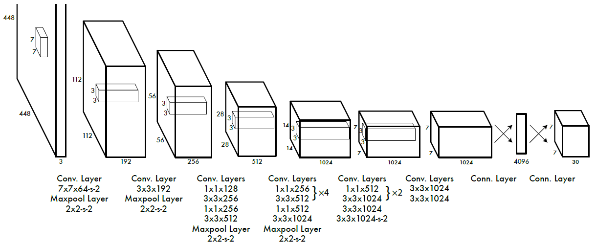
https://storage.googleapis.com/reighns/images/yolov1_model.png — Fig. 1 YoloV1 Model Architecture#

The YOLOv1 model is made up of 24 convolutional layers and 2 fully connected layers, a surprisingly simple architecture that resembles a image classification model. The authors also mentioned that the model was inspired by GoogLeNet.

We are more interested in the last layer of the network, as that is where the novelty lies. Fig. 2 is a zoomed in version of the last layer, a cuboid of shape \(7 \times 7 \times 30\). This cuboid is extremely important to understand, which we will mention more later.

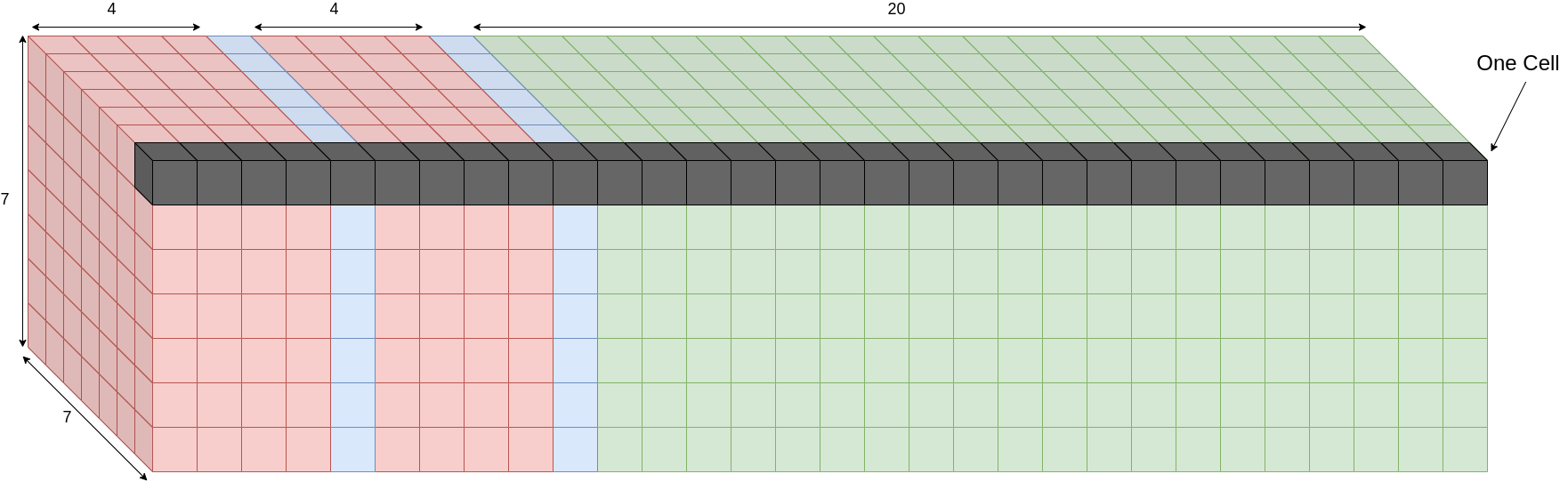
https://storage.googleapis.com/reighns/images/label_matrix.png — Fig. 2 The output tensor from YOLOv1’s last layer.#

Python Implementation#

We present a python implementation of the model in PyTorch. The implementation is modified from Aladdin Persson’s repository. In the implementation, there are some small changes such as adding batch norm layers. However, the overall architecture remains similar to what was proposed in the paper.

The model architecture in code is defined below:

from typing import List

import torch
import torchinfo
from torch import nn

class CNNBlock(nn.Module):
    """Creates CNNBlock similar to YOLOv1 Darknet architecture

    Note:
        1. On top of `nn.Conv2d` we add `nn.BatchNorm2d` and `nn.LeakyReLU`.
        2. We set `track_running_stats=False` in `nn.BatchNorm2d` because we want
           to avoid updating running mean and variance during training.
           ref: https://tinyurl.com/ap22f8nf
    """

    def __init__(self, in_channels: int, out_channels: int, **kwargs) -> None:
        """Initialize CNNBlock.

        Args:
            in_channels (int): The number of input channels.
            out_channels (int): The number of output channels.
            **kwargs (Dict[Any]): Keyword arguments for `nn.Conv2d` such as `kernel_size`,
                     `stride` and `padding`.
        """
        super().__init__()
        self.conv = nn.Conv2d(in_channels, out_channels, bias=False, **kwargs)
        self.batchnorm = nn.BatchNorm2d(
            num_features=out_channels, track_running_stats=False
        )
        self.leakyrelu = nn.LeakyReLU(negative_slope=0.1)

    def forward(self, x: torch.Tensor) -> torch.Tensor:
        """Forward pass."""
        return self.leakyrelu(self.batchnorm(self.conv(x)))


class Yolov1Darknet(nn.Module):
    def __init__(
        self,
        architecture: List,
        in_channels: int = 3,
        S: int = 7,
        B: int = 2,
        C: int = 20,
        init_weights: bool = False,
    ) -> None:
        """Initialize Yolov1Darknet.

        Note:
            1. `self.backbone` is the backbone of Darknet.
            2. `self.head` is the head of Darknet.
            3. Currently the head is hardcoded to have 1024 neurons and if you change
               the image size from the default 448, then you will have to change the
               neurons in the head.

        Args:
            architecture (List): The architecture of Darknet. See config.py for more details.
            in_channels (int): The in_channels. Defaults to 3 as we expect RGB images.
            S (int): Grid Size. Defaults to 7.
            B (int): Number of Bounding Boxes to predict. Defaults to 2.
            C (int): Number of Classes. Defaults to 20.
            init_weights (bool): Whether to init weights. Defaults to False.
        """
        super().__init__()

        self.architecture = architecture
        self.in_channels = in_channels
        self.S = S
        self.B = B
        self.C = C

        # backbone is darknet
        self.backbone = self._create_darknet_backbone()
        self.head = self._create_darknet_head()

        if init_weights:
            self._initialize_weights()

    def _initialize_weights(self) -> None:
        """Initialize weights for Conv2d, BatchNorm2d, and Linear layers."""
        for m in self.modules():
            if isinstance(m, nn.Conv2d):
                nn.init.kaiming_normal_(
                    m.weight, mode="fan_in", nonlinearity="leaky_relu"
                )
                if m.bias is not None:
                    nn.init.constant_(m.bias, 0)
            elif isinstance(m, nn.BatchNorm2d):
                nn.init.constant_(m.weight, 1)
                nn.init.constant_(m.bias, 0)
            elif isinstance(m, nn.Linear):
                nn.init.normal_(m.weight, 0, 0.01)
                nn.init.constant_(m.bias, 0)

    def forward(self, x: torch.Tensor) -> torch.Tensor:
        """Forward pass."""
        x = self.backbone(x)
        x = self.head(torch.flatten(x, start_dim=1))
        x = x.reshape(-1, self.S, self.S, self.C + self.B * 5)
        # if self.squash_type == "flatten":
        #     x = torch.flatten(x, start_dim=1)
        # elif self.squash_type == "3D":
        #     x = x.reshape(-1, self.S, self.S, self.C + self.B * 5)
        # elif self.squash_type == "2D":
        #     x = x.reshape(-1, self.S * self.S, self.C + self.B * 5)
        return x

    def _create_darknet_backbone(self) -> nn.Sequential:
        """Create Darknet backbone."""
        layers = []
        in_channels = self.in_channels

        for layer_config in self.architecture:
            # convolutional layer
            if isinstance(layer_config, tuple):
                out_channels, kernel_size, stride, padding = layer_config
                layers += [
                    CNNBlock(
                        in_channels,
                        out_channels,
                        kernel_size=kernel_size,
                        stride=stride,
                        padding=padding,
                    )
                ]
                # update next layer's in_channels to be current layer's out_channels
                in_channels = layer_config[0]

            # max pooling
            elif isinstance(layer_config, str) and layer_config == "M":
                # hardcode maxpooling layer
                layers += [nn.MaxPool2d(kernel_size=(2, 2), stride=(2, 2))]

            elif isinstance(layer_config, list):
                conv1 = layer_config[0]
                conv2 = layer_config[1]
                num_repeats = layer_config[2]

                for _ in range(num_repeats):
                    layers += [
                        CNNBlock(
                            in_channels,
                            out_channels=conv1[0],
                            kernel_size=conv1[1],
                            stride=conv1[2],
                            padding=conv1[3],
                        )
                    ]
                    layers += [
                        CNNBlock(
                            in_channels=conv1[0],
                            out_channels=conv2[0],
                            kernel_size=conv2[1],
                            stride=conv2[2],
                            padding=conv2[3],
                        )
                    ]
                    in_channels = conv2[0]

        return nn.Sequential(*layers)

    def _create_darknet_head(self) -> nn.Sequential:
        """Create the fully connected layers of Darknet head.

        Note:
            1. In original paper this should be
                nn.Sequential(
                    nn.Linear(1024*S*S, 4096),
                    nn.LeakyReLU(0.1),
                    nn.Linear(4096, S*S*(B*5+C))
                    )
            2. You can add `nn.Sigmoid` to the last layer to stabilize training
               and avoid exploding gradients with high loss since sigmoid will
               force your values to be between 0 and 1. Remember if you do not put
               this your predictions can be unbounded and contain negative numbers even.
        """

        return nn.Sequential(
            nn.Flatten(),
            nn.Linear(1024 * self.S * self.S, 4096),
            nn.Dropout(0.0),
            nn.LeakyReLU(0.1),
            nn.Linear(4096, self.S * self.S * (self.C + self.B * 5)),
            # nn.Sigmoid(),
        )

We then run a forward pass of the model as a sanity check.

batch_size = 4
image_size = 448
in_channels = 3
S = 7
B = 2
C = 20

DARKNET_ARCHITECTURE = [
    (64, 7, 2, 3),
    "M",
    (192, 3, 1, 1),
    "M",
    (128, 1, 1, 0),
    (256, 3, 1, 1),
    (256, 1, 1, 0),
    (512, 3, 1, 1),
    "M",
    [(256, 1, 1, 0), (512, 3, 1, 1), 4],
    (512, 1, 1, 0),
    (1024, 3, 1, 1),
    "M",
    [(512, 1, 1, 0), (1024, 3, 1, 1), 2],
    (1024, 3, 1, 1),
    (1024, 3, 2, 1),
    (1024, 3, 1, 1),
    (1024, 3, 1, 1),
]

x = torch.zeros(batch_size, in_channels, image_size, image_size)
y_trues = torch.zeros(batch_size, S, S, B * 5 + C)

yolov1 = Yolov1Darknet(
    architecture=DARKNET_ARCHITECTURE,
    in_channels=in_channels,
    S=S,
    B=B,
    C=C,
)

y_preds = yolov1(x)

print(f"x.shape: {x.shape}")
print(f"y_trues.shape: {y_trues.shape}")
print(f"y_preds.shape: {y_preds.shape}")

x.shape: torch.Size([4, 3, 448, 448])
y_trues.shape: torch.Size([4, 7, 7, 30])
y_preds.shape: torch.Size([4, 7, 7, 30])

The input label y_trues and y_preds are of shape (batch_size, S, S, B * 5 + C), in our case is (4, 7, 7, 30) and indeed the shape that we expected in Fig. 2. The additional first dimension is the batch size. We will talk more in the next few sections.

Model Summary#

We use torchinfo package to print out the model summary. This is a useful tool that is similar to model.summary() in Keras.

torchinfo.summary(
    yolov1, input_size=(batch_size, in_channels, image_size, image_size)
)

==========================================================================================
Layer (type:depth-idx)                   Output Shape              Param #
==========================================================================================
Yolov1Darknet                            [4, 7, 7, 30]             --
├─Sequential: 1-1                        [4, 1024, 7, 7]           --
│    └─CNNBlock: 2-1                     [4, 64, 224, 224]         --
│    │    └─Conv2d: 3-1                  [4, 64, 224, 224]         9,408
│    │    └─BatchNorm2d: 3-2             [4, 64, 224, 224]         128
│    │    └─LeakyReLU: 3-3               [4, 64, 224, 224]         --
│    └─MaxPool2d: 2-2                    [4, 64, 112, 112]         --
│    └─CNNBlock: 2-3                     [4, 192, 112, 112]        --
│    │    └─Conv2d: 3-4                  [4, 192, 112, 112]        110,592
│    │    └─BatchNorm2d: 3-5             [4, 192, 112, 112]        384
│    │    └─LeakyReLU: 3-6               [4, 192, 112, 112]        --
│    └─MaxPool2d: 2-4                    [4, 192, 56, 56]          --
│    └─CNNBlock: 2-5                     [4, 128, 56, 56]          --
│    │    └─Conv2d: 3-7                  [4, 128, 56, 56]          24,576
│    │    └─BatchNorm2d: 3-8             [4, 128, 56, 56]          256
│    │    └─LeakyReLU: 3-9               [4, 128, 56, 56]          --
│    └─CNNBlock: 2-6                     [4, 256, 56, 56]          --
│    │    └─Conv2d: 3-10                 [4, 256, 56, 56]          294,912
│    │    └─BatchNorm2d: 3-11            [4, 256, 56, 56]          512
│    │    └─LeakyReLU: 3-12              [4, 256, 56, 56]          --
│    └─CNNBlock: 2-7                     [4, 256, 56, 56]          --
│    │    └─Conv2d: 3-13                 [4, 256, 56, 56]          65,536
│    │    └─BatchNorm2d: 3-14            [4, 256, 56, 56]          512
│    │    └─LeakyReLU: 3-15              [4, 256, 56, 56]          --
│    └─CNNBlock: 2-8                     [4, 512, 56, 56]          --
│    │    └─Conv2d: 3-16                 [4, 512, 56, 56]          1,179,648
│    │    └─BatchNorm2d: 3-17            [4, 512, 56, 56]          1,024
│    │    └─LeakyReLU: 3-18              [4, 512, 56, 56]          --
│    └─MaxPool2d: 2-9                    [4, 512, 28, 28]          --
│    └─CNNBlock: 2-10                    [4, 256, 28, 28]          --
│    │    └─Conv2d: 3-19                 [4, 256, 28, 28]          131,072
│    │    └─BatchNorm2d: 3-20            [4, 256, 28, 28]          512
│    │    └─LeakyReLU: 3-21              [4, 256, 28, 28]          --
│    └─CNNBlock: 2-11                    [4, 512, 28, 28]          --
│    │    └─Conv2d: 3-22                 [4, 512, 28, 28]          1,179,648
│    │    └─BatchNorm2d: 3-23            [4, 512, 28, 28]          1,024
│    │    └─LeakyReLU: 3-24              [4, 512, 28, 28]          --
│    └─CNNBlock: 2-12                    [4, 256, 28, 28]          --
│    │    └─Conv2d: 3-25                 [4, 256, 28, 28]          131,072
│    │    └─BatchNorm2d: 3-26            [4, 256, 28, 28]          512
│    │    └─LeakyReLU: 3-27              [4, 256, 28, 28]          --
│    └─CNNBlock: 2-13                    [4, 512, 28, 28]          --
│    │    └─Conv2d: 3-28                 [4, 512, 28, 28]          1,179,648
│    │    └─BatchNorm2d: 3-29            [4, 512, 28, 28]          1,024
│    │    └─LeakyReLU: 3-30              [4, 512, 28, 28]          --
│    └─CNNBlock: 2-14                    [4, 256, 28, 28]          --
│    │    └─Conv2d: 3-31                 [4, 256, 28, 28]          131,072
│    │    └─BatchNorm2d: 3-32            [4, 256, 28, 28]          512
│    │    └─LeakyReLU: 3-33              [4, 256, 28, 28]          --
│    └─CNNBlock: 2-15                    [4, 512, 28, 28]          --
│    │    └─Conv2d: 3-34                 [4, 512, 28, 28]          1,179,648
│    │    └─BatchNorm2d: 3-35            [4, 512, 28, 28]          1,024
│    │    └─LeakyReLU: 3-36              [4, 512, 28, 28]          --
│    └─CNNBlock: 2-16                    [4, 256, 28, 28]          --
│    │    └─Conv2d: 3-37                 [4, 256, 28, 28]          131,072
│    │    └─BatchNorm2d: 3-38            [4, 256, 28, 28]          512
│    │    └─LeakyReLU: 3-39              [4, 256, 28, 28]          --
│    └─CNNBlock: 2-17                    [4, 512, 28, 28]          --
│    │    └─Conv2d: 3-40                 [4, 512, 28, 28]          1,179,648
│    │    └─BatchNorm2d: 3-41            [4, 512, 28, 28]          1,024
│    │    └─LeakyReLU: 3-42              [4, 512, 28, 28]          --
│    └─CNNBlock: 2-18                    [4, 512, 28, 28]          --
│    │    └─Conv2d: 3-43                 [4, 512, 28, 28]          262,144
│    │    └─BatchNorm2d: 3-44            [4, 512, 28, 28]          1,024
│    │    └─LeakyReLU: 3-45              [4, 512, 28, 28]          --
│    └─CNNBlock: 2-19                    [4, 1024, 28, 28]         --
│    │    └─Conv2d: 3-46                 [4, 1024, 28, 28]         4,718,592
│    │    └─BatchNorm2d: 3-47            [4, 1024, 28, 28]         2,048
│    │    └─LeakyReLU: 3-48              [4, 1024, 28, 28]         --
│    └─MaxPool2d: 2-20                   [4, 1024, 14, 14]         --
│    └─CNNBlock: 2-21                    [4, 512, 14, 14]          --
│    │    └─Conv2d: 3-49                 [4, 512, 14, 14]          524,288
│    │    └─BatchNorm2d: 3-50            [4, 512, 14, 14]          1,024
│    │    └─LeakyReLU: 3-51              [4, 512, 14, 14]          --
│    └─CNNBlock: 2-22                    [4, 1024, 14, 14]         --
│    │    └─Conv2d: 3-52                 [4, 1024, 14, 14]         4,718,592
│    │    └─BatchNorm2d: 3-53            [4, 1024, 14, 14]         2,048
│    │    └─LeakyReLU: 3-54              [4, 1024, 14, 14]         --
│    └─CNNBlock: 2-23                    [4, 512, 14, 14]          --
│    │    └─Conv2d: 3-55                 [4, 512, 14, 14]          524,288
│    │    └─BatchNorm2d: 3-56            [4, 512, 14, 14]          1,024
│    │    └─LeakyReLU: 3-57              [4, 512, 14, 14]          --
│    └─CNNBlock: 2-24                    [4, 1024, 14, 14]         --
│    │    └─Conv2d: 3-58                 [4, 1024, 14, 14]         4,718,592
│    │    └─BatchNorm2d: 3-59            [4, 1024, 14, 14]         2,048
│    │    └─LeakyReLU: 3-60              [4, 1024, 14, 14]         --
│    └─CNNBlock: 2-25                    [4, 1024, 14, 14]         --
│    │    └─Conv2d: 3-61                 [4, 1024, 14, 14]         9,437,184
│    │    └─BatchNorm2d: 3-62            [4, 1024, 14, 14]         2,048
│    │    └─LeakyReLU: 3-63              [4, 1024, 14, 14]         --
│    └─CNNBlock: 2-26                    [4, 1024, 7, 7]           --
│    │    └─Conv2d: 3-64                 [4, 1024, 7, 7]           9,437,184
│    │    └─BatchNorm2d: 3-65            [4, 1024, 7, 7]           2,048
│    │    └─LeakyReLU: 3-66              [4, 1024, 7, 7]           --
│    └─CNNBlock: 2-27                    [4, 1024, 7, 7]           --
│    │    └─Conv2d: 3-67                 [4, 1024, 7, 7]           9,437,184
│    │    └─BatchNorm2d: 3-68            [4, 1024, 7, 7]           2,048
│    │    └─LeakyReLU: 3-69              [4, 1024, 7, 7]           --
│    └─CNNBlock: 2-28                    [4, 1024, 7, 7]           --
│    │    └─Conv2d: 3-70                 [4, 1024, 7, 7]           9,437,184
│    │    └─BatchNorm2d: 3-71            [4, 1024, 7, 7]           2,048
│    │    └─LeakyReLU: 3-72              [4, 1024, 7, 7]           --
├─Sequential: 1-2                        [4, 1470]                 --
│    └─Flatten: 2-29                     [4, 50176]                --
│    └─Linear: 2-30                      [4, 4096]                 205,524,992
│    └─Dropout: 2-31                     [4, 4096]                 --
│    └─LeakyReLU: 2-32                   [4, 4096]                 --
│    └─Linear: 2-33                      [4, 1470]                 6,022,590
==========================================================================================
Total params: 271,716,734
Trainable params: 271,716,734
Non-trainable params: 0
Total mult-adds (G): 81.14
==========================================================================================
Input size (MB): 9.63
Forward/backward pass size (MB): 883.28
Params size (MB): 1086.87
Estimated Total Size (MB): 1979.78
==========================================================================================

Backbone#

We use Darknet as our backbone. The backbone serves as a feature extractor. This means that we can replace the backbone with any other feature extractor.

For example, we can replace the Darknet backbone with ResNet50, which is a 50-layer Convoluational Neural Network. You only need to make sure that the output of the backbone can match the shape of the input of the YOLO head. We often overcome the shape mismatch issue with Global Average Pooling.

Head#

Head is the part of the model that takes the output of the backbone and transforms it into the output of the model. In this case, we need to transform whatever shape we get from the backbone into the shape of the label matrix, which is (7, 7, 30).

Let’s print out the last layer(s) of the YOLOv1 model:

print(f"yolov1 last layer: {yolov1.head[-1]}")

yolov1 last layer: Linear(in_features=4096, out_features=1470, bias=True)

Unfortunately, the info is not very helpful. We will refer back to the model summary in section model summary to understand the output shape of the last layer.

Linear: 2-33                      [4, 1470]                 6,022,590

Notice that the last layer is actually a linear (fc) layer with shape [4, 1470]. This is in contrast of the output shape of y_preds which is [4, 7, 7, 30]. This is because in the forward method, we reshaped the output of the last layer to be [4, 7, 7, 30].

Why do we need to reshape the output of the last layer?

The reason of the reshape is because of better interpretation. More concretely, the paper said that the core idea is to divide the input image into an \(S \times S\) grid, where each grid cell has a shape of \(5B + C\). See Fig. 2 for a visual example.

2D matrix vs 3D tensor

If we remove the batch size dimension, then the output tensor of y_trues and y_preds will be a 3D tensor of shape (S, S, B * 5 + C) = (7, 7, 30).

We can also think of it as a 2D matrix, where we flatten the first and second dimension, essentially collapsing the \(7 \times 7\) grid into a single dimension of \(49\). The reason why I did this is for easier interpretation, as a 2D matrix is easier to visualize than a 3D tensor.

We will carry this idea forward to the next few sections.

Anchors and Prior Boxes#

Before we move on, it is beneficial to read on what anchors and prior boxes are. This will give you a better idea on why the author divide the input image into an \(S \times S\) grid.

Bounding Box Parametrization#

Before we move on, it is beneficial to read on what bounding box parametrization is. This will give you a better idea on why the author wants to transform the bounding box into offsets pertaining to the grid cell.

YOLOv1 Encoding Setup#

As a continuation of the previous section on head, we will now answer the question on why we reshape the output of the last layer to be [7, 7, 30].

The definitions of some keywords are defined in section on definitions.

Quoting from the paper:

Our system divides the input image into an S × S grid. If the center of an object falls into a grid cell, that grid cell is responsible for detecting that object [Redmon et al., 2016].

Let’s visualize this idea with the help of the diagram below.

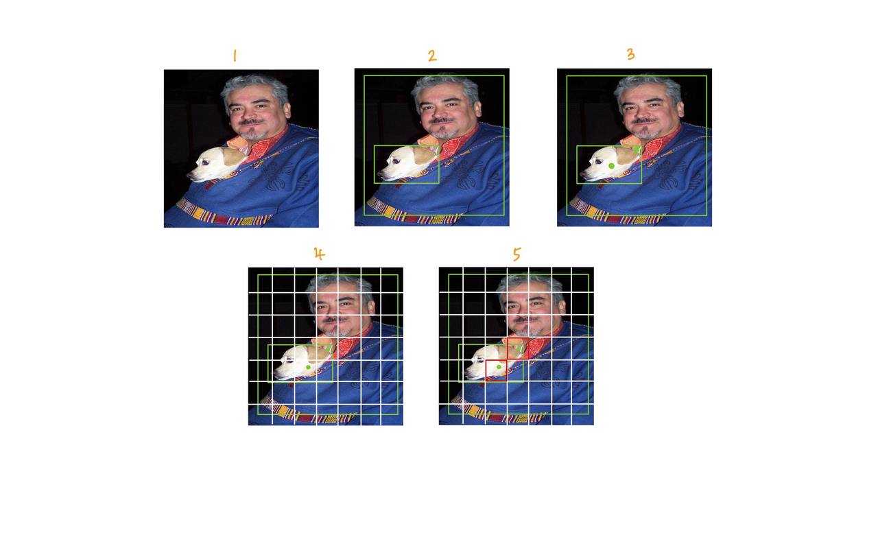
_images/yolov1_image_grids.jpg — Fig. 3 Image 1 with grids.#

Given an input image \(\X\) at part 1 of Fig. 3, we divide the image into an \(S \times S\) grid. We see there’s a person and a dog in the image.

Part 2 of Fig. 3 shows the ground truth bounding box of the object.

Part 3 of Fig. 3 adds on the center of the bounding boxes as dots.

In the case of the paper, \(S=7\) implies YOLOv1 breaks the image up into a grid of size \(7 \times 7\), as shown in part 4 of Fig. 3. The grids are drawn in white. There are a total of \(7 \times 7 = 49\) grid cells. Note the distinction between the size of the grid \(S\) and the grid cell.

These grid cells represent prior boxes so that when the network predicts box coordinates, it has something to reference them from. Remember that earlier I said whenever you predict boxes, you have to say with respect to what? Well it’s with respect to these grid cells. More concretely, the network can detect objects by predicting scales and offsets from those prior boxes.

As an illustrative example, take the prior box on the 4th row and 4th column. It’s centered on the person, so it seems reasonable that this prior box should be responsible for predicting the person in this image. The 7x7 grid isn’t actually drawn on the image, it’s just implied, and the thing that implies it is the 7x7 grid in the output tensor. You can imagine overlaying the output tensor on the image, and each cell corresponds to a part of the image. If you understand anchors, this idea should feel famililar to you [Turner, 2021].

Consequently, part 5 of Fig. 3 highlighted the “responsible” grid cell for each object in red.

So we have understood the first quote on why we divide the input image into an \(S \times S\) grid. Since the person’s center falls into the 4th row and 4th column, the grid cell at that position is then our ground truth bounding box for the person in this image. Similarly, the dog’s center falls into the 5th row and 3rd column, the grid cell at that position is then our ground truth bounding box for the dog in this image. As an aside, all other grid cells are background and we will ignore them by assigning them all zeros, more on that later.

We have answered the reason for why we need to divide the input image into an \(S \times S\) grid. Next is why there the output tensor’s shape has a 3rd dimension of depth \(B * 5 + C = 30\)?

Each grid cell predicts \(B\) bounding boxes and confidence scores for those boxes as well as \(C\) conditional class probabilities [Redmon et al., 2016].

For each grid cell \(i\), we a 30-d vector, 30 is derived from \(5 \times B + C\) elements.

So each cell is responsible for predicting boxes from a single part of the image. More specifically, each cell is responsible for predicting precisely two boxes for each part of the image. Note that there are 49 cells, and each cell is predicting two boxes, so the whole network is only going to predict 98 boxes. That number is fixed.

In order to predict a single box, the network must output a number of things. Firstly it must encode the coordinates of the box which YOLO encodes as (x, y, w, h), where x and y are the center of the box. Earlier I suggested you familiarise yourself with box parameterisation, this is because YOLO does not output the actual coordinates of the box, but parameterised coordinates instead. Firstly, the width and height are normalised with respect to the image width, so if the network outputs a value of 1.0 for the width, it’s saying the box should span the entire image, likewise 0.5 means it’s half the width of the image. Note that the width and height have nothing to do with the actual grid cell itself. The x and y values are parameterised with respect to the grid cell, they represent offsets from the grid cell position. The grid cell has a width and height which is equal to 1/S (we’ve normalised the image to have width and height 1.0). If the network outputs a value of 1.0 for x, then it’s saying that the x value of the box is the x position of the grid cell plus the width of the grid cell.

Secondly, YOLO also predicts a confidence score for each box which represents the probability that the box contains an object. Lastly, YOLO predicts a class, which is represented by a vector of C values, and the predicted class is the one with the highest value. Now, here’s the catch. YOLO does not predict a class for every box, it predicts a class for each cell. But each cell is associated with two boxes, so those boxes will have the same predicted class, even though they may have different shapes and positions. Let’s tie all that together visually, let me copy down my diagram again.

The first five values encode the location and confidence of the first box, the next five encode the location and confidence of the next box, and the final 20 encode the 20 classes (because Pascal VOC has 20 classes). In total, the size of the vector is 5xB + C where B is the number of boxes, and C is the number of classes.

The way that YOLO actually predicts boxes, is by predicting target scale and offset values for each prior, these are parameterised by normalising by the width and height of the image. For example, take the highlighted top right cell in the output tensor, this particular cell corresponds to the far top right cell in the input image (which looks like the branch of a tree). That cell represents a prior box, which will have a width and height equal to the image width divided by 7 and image height divided by 7 respectively, and the location being the top right. The outputs from this single cell will therefore shift and stretch that prior box into new positions that hopefully contain the object.

Because the cell predicts two boxes, it will shift and stretch the prior box in two different ways, possibly to cover two different objects (but both are constrained to have the same class). You might wonder why it’s trying to do two boxes. The answer is probably because 49 boxes isn’t enough, especially when there are lots of objects close together, although what tends to happen during training is that the predicted boxes become specialised. So one box might learn to find big things, the other might learn to find small things, this may help the network generalise to other domains.

To wrap this section up, I want to point out one difference between the approach that YOLO has taken, and the anchor boxes in the Region Proposal Network. Anchors in the RPN actually refer to the nine different aspect ratios and scales from a single location. In other words, each position in the RPN predicts nine different boxes from nine different prior widths and heights. In contrast, it’s as if YOLO has two anchors at each position, but they have the same width and height. YOLO does not introduce variations in aspect ratio or size into the anchor boxes.

As a final note to help your intuition, it’s reasonable to wonder why they didn’t predict a class for each box. What would the output look like? You’d still have 7x7 cells, but instead of each cell being of size 5xB + C, you’d have (5+C) x B. So for two boxes, you’d have 50 outputs, not 30. That doesn’t seem unreasonable, and it gives the network the flexibility to predict two different classes from the same location.

Notations and Definitions#

Sample Image#

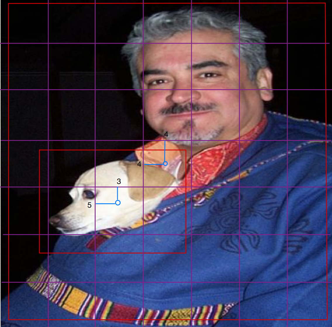
https://storage.googleapis.com/reighns/images/grid_on_image.PNG — Fig. 5 Sample Image with Grids.#

Bounding Box Parametrization#

Given a yolo format bounding box, we will perform parametrization to transform the coordinates of the bounding box to a more convenient form. Before that, let us define some notations.

Definition 1 (YOLO Format Bounding Box)

The YOLO format bounding box is a 4-tuple vector consisting of the coordinates of the bounding box in the following order:

(1)#\[ \byolo = \begin{bmatrix} \xx_c & \yy_c & \ww_n & \hh_n \end{bmatrix} \in \R^{1 \times 4} \]

where

\(\xx_c\) and \(\yy_c\) are the coordinates of the center of the bounding box, normalized with respect to the image width and height;
\(\ww_n\) and \(\hh_n\) are the width and height of the bounding box, normalized with respect to the image width and height.

Consequently, all coordinates are in the range \([0, 1]\).

We could be done at this step and ask the model to predict the bounding box in YOLO format. However, the author proposes a more convenient parametrization for the model to learn better:

The center of the bounding box is parametrized as the offset from the top-left corner of the grid cell to the center of the bounding box. We will go through an an example later.
The width and height of the bounding box are parametrized to the square root of the width and height of the bounding box.

Intuition: Parametrization of Bounding Box

The loss function of YOLOv1 is using mean squared errror.

The square root is present so that errors in small bounding boxes are more penalizing than errors in big bounding boxes. Recall that square root mapping expands the range of small values for values between \(0\) and \(1\).

For example, if the normalized width and height of a bounding box is \([0.05, 0.8]\) respectively, it means that the bounding box’s width is 5% of the image width and height is 80% of the image height. We can scale it back since absolute numbers are easier to visualize.

Given an image of size \(100 \times 100\), the bounding box’s width and height unnormalized are \(5\) and \(80\) respectively. Then let’s say the model predicts the bounding box’s width and height to be \([0.2, 0.95]\). The mean squared error is \((0.2 - 0.05)^2 + (0.95 - 0.8)^2 = 0.0225 + 0.0225 = 0.045\). We see that both errors are penalized equally. But if you scale the predicted bounding box’s width and height back to the original image size, you will get \(20\) and \(95\) respectively, then the relative error is much worse for the width than the height (i.e both deviates 15 pixels but the width deviates much more percentage wise).

Consequently, the square root mapping is used to penalize errors in small bounding boxes more than the errors in big bounding boxes. If we use square root mapping, our original width and height becomes \([0.22, 0.89]\) and the predicted width and height becomes \([0.45, 0.97]\). The mean squared error is then \((0.45 - 0.22)^2 + (0.97 - 0.89)^2 = 0.0529 + 0.0064 = 0.0593\). We see that the error in the width is penalized more than the error in the height. This helps the model to learn better by assigning more importance to small bounding boxes errors.

Definition 2 (Parametrized Bounding Box)

The parametrized bounding box is a 4-tuple vector consisting of the coordinates of bounding box in the following order:

(2)#\[ \b = \begin{bmatrix} f(\xx_c, \gx) & f(\yy_c, \gy) & \sqrt{\ww_n} & \sqrt{\hh_n} \end{bmatrix} \in \R^{1 \times 4} \]

where

\(\gx = \lfloor S \cdot \xx_c \rfloor\) is the grid cell column (row) index;
\(\gy = \lfloor S \cdot \yy_c \rfloor\) is the grid cell row (column) index;
\(f(\xx_c, \gx) = S \cdot \xx_c - \gx\) and;
\(f(\yy_c, \gy) = S \cdot \yy_c - \gy\)

Take note that during construction, the square root is omitted because it is included in the loss function later. You will see in our code later that our \(\b\) is actually

\[\begin{split} \begin{align} \b &= \begin{bmatrix} f(\xx_c, \gx) & f(\yy_c, \gy) & \ww_n & \hh_n \end{bmatrix} \\ &= \begin{bmatrix} \xx & \yy & \ww & \hh \end{bmatrix} \end{align} \end{split}\]

We will be using the notation \([\xx, \yy, \ww, \hh]\) in the rest of the sections.

As a side note, it is often the case that a single image has multiple bounding boxes. Therefore, you will need to convert all of them to the parametrized form.

Example 1 (Example of Parametrization)

Consider the TODO insert image image. The bounding box is in the YOLO format at first.

\[ \byolo = \begin{bmatrix} 11 & 0.3442 & 0.611 & 0.4164 & 0.262 \end{bmatrix} \]

Then since \(S = 7\), we can recover \(f(\xx_c, \gx)\) and \(f(\yy_c, \gy)\) as follows:

\[\begin{split} \begin{aligned} \gx &= \lfloor 7 \cdot 0.3442 \rfloor &= 2 \\ \gy &= \lfloor 7 \cdot 0.611 \rfloor &= 4 \\ f(\xx_c, \gx) &= 7 \cdot 0.3442 - 2 &= 0.4093 \\ f(\yy_c, \gy) &= 7 \cdot 0.611 - 4 &= 0.2770 \\ \end{aligned} \end{split}\]

Visually, the bounding box of the dog actually lies in the 3rd column and 5th row \((3, 5)\) of the grid. But we compute it as if it lies in the 2nd column and 4th row \((2, 4)\) of the grid because in python the index starts from 0 and the top-left corner of the image is considered grid cell \((0, 0)\).

Then the parametrized bounding box is:

\[ \b = \begin{bmatrix} 0.4093 & 0.2770 & \sqrt{0.4164} & \sqrt{0.262} \end{bmatrix} \in \R^{1 \times 4} \]

For more details, have a read at this article to understand the parametrization.

Loss Function#

See below section.

Other Important Notations#

Definition 3 (S, B and C)

\(S\): We divide an image into an \(S \times S\) grid, so \(S\) is the grid size;
\(\gx\) denotes \(x\)-coordinate grid cell and \(\gy\) denotes the \(y\)-coordinate grid cell and so the first grid cell can be denoted \((\gx, \gy) = (0, 0)\) or \((1, 1)\) if using python;
\(B\): In each grid cell \((\gx, \gy)\), we can predict \(B\) number of bounding boxes;
\(C\): This is the number of classes;
Let \(\cc \in \{1, 2, \ldots, 20\}\) be a scalar, which is the class index (id) where
- 20 is the number of classes;
- in Pascal VOC: [aeroplane, bicycle, bird, boat, bottle, bus, car, cat, chair, cow, diningtable, dog, horse, motorbike, person, pottedplant, sheep, sofa, train, tvmonitor]
- So if the object is class bicycle, then \(\cc = 2\);
- Note in python notation, \(\cc\) starts from \(0\) and ends at \(19\) so need to shift accordingly.

Definition 4 (Probability Object)

The author defines \(\Pobj\) to be the probability that an object is present in a grid cell. This is constructed deterministically to be either \(0\) or \(1\).

To make the notation more compact, we will add a subscript \(i\) to denote the grid cell.

\[\begin{split} \Pobj_i = \begin{cases} 1 & \textbf{if grid cell } i \textbf{ has an object}\\ 0 & \textbf{otherwise} \end{cases} \end{split}\]

By definition, if a ground truth bounding box’s center coordinates \((\xx_c, \yy_c)\) falls in grid cell \(i\), then \(\Pobj_i = 1\) for that grid cell.

Definition 5 (Ground Truth Confidence Score)

The author defines the confidence score of the ground truth matrix to be

\[ \conf_i = \Pobj_i \times \iou \]

where

\[\iou = \underset{\bhat_i \in \{\bhat_i^1, \bhat_i^2\}}{\max}\textbf{IOU}(\b_i, \bhat_i)\]

where \(\bhat_i^1\) and \(\bhat_i^2\) are the two bounding boxes that are predicted by the model.

It is worth noting to the readers that \(\conf_i\) is also an indicator function, since \(\Pobj_i\) from Definition 4 is an indicator function.

More concretely,

\[\begin{split} \conf_i = \begin{cases} \textbf{IOU}(\b_i, \bhat_i) & \textbf{if grid cell } i \textbf{ has an object}\\ 0 & \textbf{otherwise} \end{cases} \end{split}\]

since \(\Pobj_i = 1\) if the grid cell has an object and \(\Pobj_i = 0\) otherwise.

Therefore, the author is using the IOU as a proxy for the confidence score in the ground truth matrix.

From 3D Tensor to 2D Matrix#

We will now discuss how to convert the 3D tensor output of the YOLOv1 model to a 2D matrix.

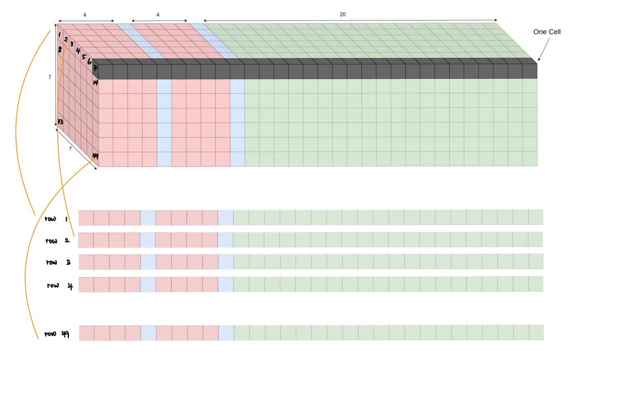
_images/3dto2d.jpg — Fig. 6 Convert 3D tensor to 2D matrix#

Recall that the output of the YOLOv1 model is a 3D tensor of shape \((7, 7, 30)\) for a single image (not including batch size). Visually, Fig. 3 shows the \(7\) by \(7\) grid overlayed on the image, each grid will have a depth of \(30\). However, when computing the loss function, I took the liberty to squash the \(7 \times 7\) grid into a single dimension, so instead of a cuboid, we now have a 2d rectangular matrix of shape \(49 \times 30\).

Construction of Ground Truth Matrix#

Abuse of Notation

When I say grid cell \(i\), it also means the \(i\)-th row of the ground truth and prediction matrix.

The below shows an image alongside its bounding boxes, in YOLO format as per Definition 1.

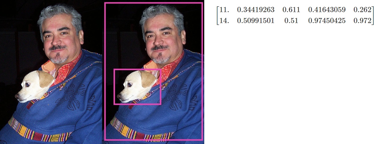
_images/image_1_and_bbox_and_labels.jpg — Fig. 7 Image 1 and its yolo format label.#

Here we see this image has 2 bounding boxes, and each bounding box has 5 values, which corresponds to the 5 values in the YOLO format.

Our goal here is to convert the YOLO style labels into a \(49 \times 30\) matrix (equivalent to a 3D tensor of shape \(7 \times 7 \times 30\)).

Recall that in section bounding box parametrization, we mentioned that YOLOv1 predicts the offset for its bounding box center, and the square root of width and height. And recall that the ground truth bounding box’s center determines which grid cell it belongs to, this is particularly important to remember.

More formally, we denote the subscript \(i\) to be the \(i\)-th grid cell where \(i \in \{1, 2, \ldots 49\}\) as seen in Fig. 6.

We will assume \(S=7\), \(B=2\), and \(C=20\), where

\(S\) is the grid size;
\(B\) is the number of bounding boxes to be predicted;
\(C\) is the number of classes.

We will also assume that our batch size is \(1\), and hence we are only looking at one single image. This simplifies the explanation. Just note that if we have a batch size of \(N\), then we will have \(N\) ground truth matrices.

Consequently, each row of the ground truth matrix will have \(2B + C = 30\) elements.

Remember that each row \(i\) of the ground truth matrix corresponds to the grid cell \(i\) as seen in figure Fig. 6.

Definition 6 (YOLOv1 Ground Truth Matrix)

Define \(\y_i \in \R^{1 \times 30}\) to be the \(i\)-th row of the ground truth matrix \(\y \in \R^{49 \times 30}\).

(3)#\[ \y_i = \begin{bmatrix} \b_i & \conf_i & \b_i & \conf_i & \p_i \end{bmatrix} \in \R^{1 \times 30} \]

where

\(\b_i = \begin{bmatrix}\xx_i & \yy_i & \ww_i & \hh_i \end{bmatrix} \in \R^{1 \times 4}\) as per Definition 2;
\(\conf_i = \Pobj_i \cdot \iou \in \R\) as per Definition 5, note very carefully how \(\conf_i\) is defined if the grid cell has an object, and how it is \(0\) if there are no objects in that grid cell \(i\).
- We will keep the formal definition off the tables for now and set \(\conf_i\) to be equals to \(\Pobj_i\) such that \(\conf = 1\) if \(\Pobj_i = 1\) and \(0\) if \(\Pobj_i = 0\).
- The reason is non-trivial because we have no way of knowing the IOU of the ground truth bounding box with the predicted bounding box before training. You can think of it as a proxy for the calculation later during the loss function construction.
\(\p_i = \begin{bmatrix}0 & 0 & 1 & \cdots &0\end{bmatrix} \in \R^{1 \times 20}\) where we use the class id \(\cc\) to construct our class probability ground truth vector such that \(\p\) is everywhere \(0\) encoded except at the \(\cc\)-th index (one hot encoding). In the paper, \(\p_i\) is defined as \(\P(\text{Class}_i \mid \text{Obj})\) which means that \(\p_i\) is conditioned on the grid cell given there exists an object, which means for grid cells \(i\) without any objects, \(\p_i\) is a zero vector.

\(\y_i\) will be initiated as a zero vector, and will remain a zero vector if there are no objects in grid cell \(i\). Otherwise, we will update the elements of \(\y_i\) as per the above definitions.

Then the ground truth matrix \(\y\) is constructed as follows:

\[\begin{split} \y = \begin{bmatrix} \y_1 \\ \y_2 \\ \vdots \\ \y_{49} \end{bmatrix} \in \R^{49 \times 30} \end{split}\]

Note that this is often reshaped to be \(\y \in \R^{7 \times 7 \times 30}\) in many implementations.

Remark 1 (Remark: Ground Truth Matrix Construction)

TODO insert encode here to show why the 1st 5 and next 5 elements are the same

It is also worth noting to everyone that we set the first 5 elements and the next 5 elements the same, therefore, we don’t make a conscious effort to differentiate between \(\b_i\), as we will see later in the prediction matrix. This is because we only have one set of ground truth and our choice of encoding is simply to repeat the ground truth coordinates twice in the first 10 elements.

The next thing to note is that what if the same image has 2 bounding boxes having the same center coordinates? Then by design, one of them will be dropped by this construction, this kind of “flawed design” will be fixed in future yolo iterations.

One can read how it is implemented in python under the encode function. The logic should follow through.

One more note is for example the dog/human image, there are two bounding boxes in that image, and one can see their center lie in different grid cells, which means the final \(7 \times 7 \times 30\) matrix will have grid cell \((3, 5)\) and \((4, 4)\) filled with values of these two bounding boxes and rest are initiated with zeros since there does not exist any objects in the other grid cells. If you are using \(49 \times 30\) method, then they instead like in grid cell \(3 \times 7 + 5 = 26\) grid cell and \(4 \times 7 + 4 = 32\) grid cell (note it is not just 3 x 5 or 4 x 4 !)

Lastly, the idea of having 2 bounding boxes in the encoding construction will be more apparent in the next section.

Construction of Prediction Matrix#

Abuse of Notation

When I say grid cell \(i\), it also means the \(i\)-th row of the ground truth and prediction matrix.

The construction of the prediction matrix \(\hat{\y}\) follows the last layer of the neural network, shown earlier in diagram YoloV1 Model Architecture.

To stay consistent with the shape defined in Definition 6, we will reshape the last layer from \(7 \times 7 \times 30\) to \(49 \times 30\). As mentioned in the section on model’s head the last layer is not really a 3d-tensor, it is in fact a linear/dense layer of shape \([-1, 1470]\). The \(1470\) neurons were reshaped to be \(7 \times 7 \times 30\) so that readers like us can interpret it better with the injection of grid cell idea.

Definition 7 (YOLOv1 Prediction Matrix)

Define \(\hat{\y}_i \in \R^{1 \times 30}\) to be the \(i\)-th row of the prediction matrix \(\hat{\y} \in \R^{49 \times 30}\), output from the last layer of the neural network.

(4)#\[ \yhat_i = \begin{bmatrix} \bhat_i^1 & \confhat_i^1 & \bhat_i^2 & \confhat_i^2 & \phat_i \end{bmatrix} \in \R^{1 \times 30} \]

where

\(\bhat_i^1 = \begin{bmatrix}\xxhat_i^1 & \yyhat_i^1 & \wwhat_i^1 & \hhhat_i^1 \end{bmatrix} \in \R^{1 \times 4}\) is the predictions of the 4 coordinates made by bounding box 1;
\(\bhat_i^2\) is then the predictions of the 4 coordinates made by bounding box 2;
\(\confhat_i^1 \in \R\) is the object/bounding box confidence score (a scalar) of the first bounding box made by the model. As a reminder, this value will be compared during loss function with the \(\conf\) constructed in the ground truth;
\(\confhat_i^2 \in \R\) is the object/bounding box confidence score of the second bounding box made by the model;
\(\phat_i \in \R^{1 \times 20}\) where the model predicts a class probability vector indicating which class is the most likely. By construction of loss function, this probability vector does not sum to 1 since the author uses MSELoss to penalize, this is slightly counter intuitive as cross-entropy loss does a better job at forcing classification loss - this is remedied in later yolo versions!
- Notice that there is no superscript for \(\phat_i\), that is because the model only predicts one set of class probabilities for each grid cell \(i\), even though you can predict \(B\) number of bounding boxes.

Consequently, the final form of the prediction matrix \(\yhat\) can be denoted as

\[\begin{split} \yhat = \begin{bmatrix} \yhat_1 \\ \yhat_2 \\ \vdots \\ \yhat_{49} \end{bmatrix} \in \R^{49 \times 30} \end{split}\]

and of course they must be the same shape as \(\y\).

Some Remarks

Note that in our head layer, we did not choose to add nn.Sigmoid() after the last layer. This will cause the output of the last layer to be in the range of \([-\infty, \infty]\), which means it is unbounded. Therefore, non-negative values like the width and height what_i and hhat_i can be negative!
Each grid cell predicts two bound boxes, it will shift and stretch the prior box in two different ways, possibly to cover two different objects (but both are constrained to have the same class). You might wonder why it’s trying to do two boxes. The answer is probably because 49 boxes isn’t enough, especially when there are lots of objects close together, although what tends to happen during training is that the predicted boxes become specialised. So one box might learn to find big things, the other might learn to find small things, this may help the network generalise to other domains1.

Loss Function#

Possibly the most important part of the YOLOv1 paper is the loss function, it is also the most confusing if you are not familiar with the notation.

We will use the first batch of images to illustrate the loss function, the batch size is 4.

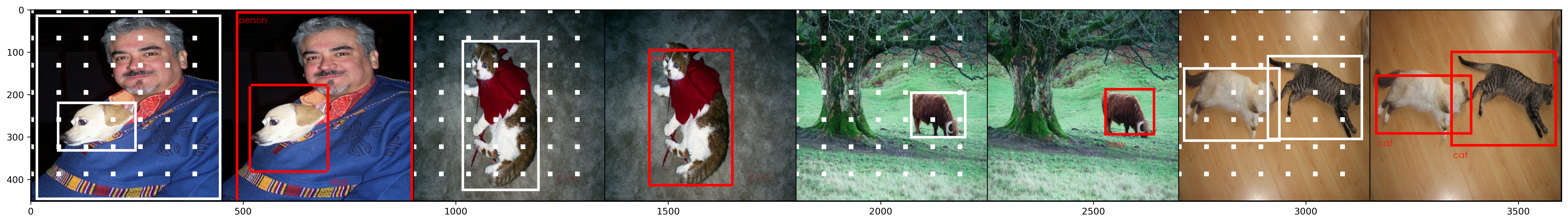
_images/batch_image.png — Fig. 8 The first 4 images.#

We will encode the 4 ground truth images in the first batch into the ground truth matrix \(\y\). Subsequently, we will pass the first batch of images to our model defined in the model section and obtain the prediction matrix \(\hat{\y}\).

Abuse of Notation

In Definition 6 and Definition 7, \(\y\) and \(\hat{\y}\) are 2 dimensional matrices with shape \(49 \times 30\). Here, we are loading 4 images, so the shape of \(\y\) and \(\hat{\y}\) will be \(4 \times 49 \times 30\).

I directly saved the ground truth matrix \(\y\) and prediction matrix \(\yhat\) as y_trues.pt and y_preds.pt respectively, you can load them with torch.load and they are in the shape of [4, 7, 7, 30]. This means that there are 4 images in the batch, each image has a ground truth matrix of shape [7, 7, 30] and a prediction matrix of shape [7, 7, 30]. The 4 images are the first 4 images in our first batch of the train loader, as illustrated in Fig. 8.

# load directly the first batch of the train loader
device = torch.device("cuda" if torch.cuda.is_available() else "cpu")
y_trues = torch.load("./assets/y_trues.pt", map_location=device)
y_preds = torch.load("./assets/y_preds.pt", map_location=device)
print(f"y_trues.shape: {y_trues.shape}")
print(f"y_preds.shape: {y_preds.shape}")

y_trues.shape: torch.Size([4, 7, 7, 30])
y_preds.shape: torch.Size([4, 7, 7, 30])

To be consistent with our notation and definition in Definition 6 and Definition 7, we will only use the first image in the batch, y_true = y_trues[0] and y_pred = y_preds[0] and reshape them to be [49, 30] and [49, 30] respectively. Thus, y_true corresponds to the ground truth matrix \(\y\) and y_pred corresponds to the prediction matrix \(\hat{\y}\).

Both of these matrix are reshaped to \(49 \times 30\) and visualized as a pandas dataframe:

	x_i^1	y_i^1	w_i^1	h_i^1	conf_i^1	x_i^2	y_i^2	w_i^2	h_i^2	conf_i^2	p_12	p_15
0	0.000	0.000	0.000	0.000	0	0.000	0.000	0.000	0.000	0	0	0
1	0.000	0.000	0.000	0.000	0	0.000	0.000	0.000	0.000	0	0	0
2	0.000	0.000	0.000	0.000	0	0.000	0.000	0.000	0.000	0	0	0
3	0.000	0.000	0.000	0.000	0	0.000	0.000	0.000	0.000	0	0	0
4	0.000	0.000	0.000	0.000	0	0.000	0.000	0.000	0.000	0	0	0
5	0.000	0.000	0.000	0.000	0	0.000	0.000	0.000	0.000	0	0	0
6	0.000	0.000	0.000	0.000	0	0.000	0.000	0.000	0.000	0	0	0
7	0.000	0.000	0.000	0.000	0	0.000	0.000	0.000	0.000	0	0	0
8	0.000	0.000	0.000	0.000	0	0.000	0.000	0.000	0.000	0	0	0
9	0.000	0.000	0.000	0.000	0	0.000	0.000	0.000	0.000	0	0	0
10	0.000	0.000	0.000	0.000	0	0.000	0.000	0.000	0.000	0	0	0
11	0.000	0.000	0.000	0.000	0	0.000	0.000	0.000	0.000	0	0	0
12	0.000	0.000	0.000	0.000	0	0.000	0.000	0.000	0.000	0	0	0
13	0.000	0.000	0.000	0.000	0	0.000	0.000	0.000	0.000	0	0	0
14	0.000	0.000	0.000	0.000	0	0.000	0.000	0.000	0.000	0	0	0
15	0.000	0.000	0.000	0.000	0	0.000	0.000	0.000	0.000	0	0	0
16	0.000	0.000	0.000	0.000	0	0.000	0.000	0.000	0.000	0	0	0
17	0.000	0.000	0.000	0.000	0	0.000	0.000	0.000	0.000	0	0	0
18	0.000	0.000	0.000	0.000	0	0.000	0.000	0.000	0.000	0	0	0
19	0.000	0.000	0.000	0.000	0	0.000	0.000	0.000	0.000	0	0	0
20	0.000	0.000	0.000	0.000	0	0.000	0.000	0.000	0.000	0	0	0
21	0.000	0.000	0.000	0.000	0	0.000	0.000	0.000	0.000	0	0	0
22	0.000	0.000	0.000	0.000	0	0.000	0.000	0.000	0.000	0	0	0
23	0.000	0.000	0.000	0.000	0	0.000	0.000	0.000	0.000	0	0	0
24	0.569	0.570	0.975	0.972	1	0.569	0.570	0.975	0.972	1	0	1
25	0.000	0.000	0.000	0.000	0	0.000	0.000	0.000	0.000	0	0	0
26	0.000	0.000	0.000	0.000	0	0.000	0.000	0.000	0.000	0	0	0
27	0.000	0.000	0.000	0.000	0	0.000	0.000	0.000	0.000	0	0	0
28	0.000	0.000	0.000	0.000	0	0.000	0.000	0.000	0.000	0	0	0
29	0.000	0.000	0.000	0.000	0	0.000	0.000	0.000	0.000	0	0	0
30	0.409	0.277	0.416	0.262	1	0.409	0.277	0.416	0.262	1	1	0
31	0.000	0.000	0.000	0.000	0	0.000	0.000	0.000	0.000	0	0	0
32	0.000	0.000	0.000	0.000	0	0.000	0.000	0.000	0.000	0	0	0
33	0.000	0.000	0.000	0.000	0	0.000	0.000	0.000	0.000	0	0	0
34	0.000	0.000	0.000	0.000	0	0.000	0.000	0.000	0.000	0	0	0
35	0.000	0.000	0.000	0.000	0	0.000	0.000	0.000	0.000	0	0	0
36	0.000	0.000	0.000	0.000	0	0.000	0.000	0.000	0.000	0	0	0
37	0.000	0.000	0.000	0.000	0	0.000	0.000	0.000	0.000	0	0	0
38	0.000	0.000	0.000	0.000	0	0.000	0.000	0.000	0.000	0	0	0
39	0.000	0.000	0.000	0.000	0	0.000	0.000	0.000	0.000	0	0	0
40	0.000	0.000	0.000	0.000	0	0.000	0.000	0.000	0.000	0	0	0
41	0.000	0.000	0.000	0.000	0	0.000	0.000	0.000	0.000	0	0	0
42	0.000	0.000	0.000	0.000	0	0.000	0.000	0.000	0.000	0	0	0
43	0.000	0.000	0.000	0.000	0	0.000	0.000	0.000	0.000	0	0	0
44	0.000	0.000	0.000	0.000	0	0.000	0.000	0.000	0.000	0	0	0
45	0.000	0.000	0.000	0.000	0	0.000	0.000	0.000	0.000	0	0	0
46	0.000	0.000	0.000	0.000	0	0.000	0.000	0.000	0.000	0	0	0
47	0.000	0.000	0.000	0.000	0	0.000	0.000	0.000	0.000	0	0	0
48	0.000	0.000	0.000	0.000	0	0.000	0.000	0.000	0.000	0	0	0

	xhat_i^1	yhat_i^1	what_i^1	hhat_i^1	confhat_i^1	xhat_i^2	yhat_i^2	what_i^2	hhat_i^2	confhat_i^2	phat_1	phat_2	phat_3	phat_4	phat_5	phat_6	phat_7	phat_8	phat_9	phat_10	phat_11	phat_12	phat_13	phat_14	phat_15	phat_16	phat_17	phat_18	phat_19	phat_20
0	0.925	-0.167	0.191	0.723	2.136e-01	1.001	0.123	0.058	0.562	-0.119	-0.586	-0.023	-0.102	-0.160	-0.408	0.564	-0.163	0.294	-0.206	-0.684	-0.215	0.340	0.425	0.139	-0.416	-0.233	0.282	0.517	0.394	0.067
1	0.333	0.190	-0.084	0.428	-2.902e-01	-0.190	0.359	0.036	-0.130	-0.684	0.415	-0.072	-0.182	0.325	0.034	-0.096	-0.258	-0.180	-0.489	-0.192	0.040	0.550	0.492	0.279	-0.157	-0.329	-0.106	0.201	-0.394	-0.536
2	-0.357	0.445	0.691	-0.301	-3.701e-01	0.430	0.238	0.456	-0.005	0.113	0.245	0.247	0.007	-0.348	0.301	-0.747	-0.056	-0.194	0.124	-0.437	0.172	0.239	-0.426	0.208	0.255	0.335	-0.152	-0.526	-0.571	0.732
3	0.120	-0.016	0.732	-0.233	-4.154e-02	0.428	-0.482	0.158	-0.246	0.008	0.007	-0.134	-0.639	-0.528	-0.545	-0.689	0.001	0.037	0.306	-0.073	0.491	-1.053	-0.516	-0.011	-0.237	0.480	-0.823	0.418	-0.284	0.166
4	-0.530	-0.381	0.081	-0.241	-3.752e-03	0.144	0.989	-0.177	0.247	0.254	0.082	0.023	-0.102	0.011	0.217	0.497	0.224	0.241	-0.125	0.143	0.318	0.057	-0.001	-0.278	-0.100	-0.022	-0.320	-0.012	-0.473	-0.214
5	-0.367	0.217	0.163	0.474	3.846e-02	0.819	0.911	-0.328	-0.047	-0.169	0.276	0.370	-0.223	0.452	-0.117	-0.101	0.521	0.543	0.128	0.347	-0.242	-0.280	-0.414	-0.296	0.662	-0.016	-0.429	0.006	-0.033	0.192
6	0.056	-0.261	-0.041	-0.109	-4.398e-01	0.329	0.178	-0.114	0.438	-0.139	-0.394	0.267	0.391	-0.533	0.146	0.357	0.239	-0.165	-0.399	0.138	0.357	0.368	-0.390	-0.063	0.536	0.388	0.494	-0.719	0.554	-0.684
7	-0.323	-0.115	-0.155	-0.017	-5.969e-02	-0.324	0.163	0.098	0.368	-0.294	0.195	0.213	-0.606	0.530	0.527	0.623	-0.519	-0.168	0.006	-0.098	0.550	-0.658	0.092	-0.250	0.283	-0.299	0.028	0.308	0.108	-0.388
8	0.058	-0.061	0.219	-0.263	-1.409e-01	-0.413	1.218	0.328	-0.635	0.053	0.021	0.107	-0.358	-0.160	-0.074	0.215	0.065	0.347	-0.394	0.225	-0.056	0.299	0.251	-0.041	0.250	0.526	-0.049	-0.105	-0.047	0.449
9	-0.203	0.044	-0.260	-0.105	-1.989e-01	0.513	0.673	-0.081	-0.436	0.098	-0.065	0.443	0.228	-0.377	-0.392	0.062	0.130	-0.444	-0.184	-0.444	0.390	-0.070	0.167	-0.247	0.537	0.262	0.460	-0.112	0.332	0.022
10	0.238	0.411	-0.264	-0.063	-3.446e-01	-0.468	-0.379	-0.382	0.066	-0.019	0.330	-0.013	-0.436	0.677	-0.064	-0.539	0.522	0.236	-0.458	0.315	0.715	-0.603	-0.656	0.243	-0.438	0.360	-0.120	-0.199	0.668	-0.379
11	0.088	0.015	-0.039	0.089	8.807e-04	0.047	0.180	0.015	0.551	-0.589	0.366	0.779	0.066	0.002	-0.246	-0.187	-0.101	-0.064	-0.061	-0.185	0.833	-0.086	0.148	-0.872	-0.028	-0.332	0.629	-0.334	0.074	-0.261
12	-0.696	0.406	0.131	0.442	2.473e-01	0.346	0.212	0.511	0.261	-0.268	0.843	0.509	0.369	0.157	0.678	0.062	0.338	0.233	0.043	-0.484	0.741	0.894	0.248	-0.087	0.459	0.017	0.316	0.255	-0.019	0.087
13	-0.929	0.255	0.358	0.456	2.613e-01	0.114	-0.744	0.038	-0.050	-0.090	-0.079	0.846	-0.015	-0.195	-0.542	-0.793	0.091	0.340	0.454	-0.159	-0.206	-0.405	-0.869	0.209	-0.464	-0.476	-0.498	0.077	0.125	0.794
14	-0.256	-0.506	0.134	-0.352	1.512e-01	-0.156	0.459	0.003	0.396	0.045	0.563	-0.141	0.418	-0.167	0.270	-0.238	0.416	0.160	0.144	0.170	-0.024	-0.285	0.368	0.608	0.626	0.444	0.312	-0.195	0.312	-0.177
15	0.627	-0.240	-0.348	-0.289	-1.770e-01	0.407	0.771	0.890	0.773	0.266	0.277	-0.003	0.392	0.296	-0.704	-0.073	0.464	-0.375	-0.123	0.335	0.818	0.108	0.300	0.042	0.247	-0.042	0.103	0.063	-0.433	-0.014
16	-0.128	0.017	-0.486	-0.198	1.439e-01	0.089	-0.336	0.091	0.735	0.257	-0.166	0.179	-0.143	-0.146	-0.147	-0.181	0.783	-0.271	-0.275	-0.407	-0.366	-0.667	-0.326	0.114	0.101	-0.164	-1.082	0.694	0.254	0.340
17	-0.156	-0.408	-0.223	-0.094	1.400e-01	0.829	1.379	-0.280	-1.207	0.340	-0.236	-0.458	-0.165	0.690	0.432	-0.300	0.104	0.311	-0.302	0.112	0.182	-0.267	-0.387	-0.137	0.476	-0.040	-0.070	0.232	-0.208	0.206
18	-0.208	-0.629	0.139	-0.178	1.545e-01	0.104	-0.012	-0.480	-0.259	-0.010	-0.117	0.114	-0.057	-0.348	-0.097	0.329	0.122	0.006	-0.043	0.091	-0.165	0.039	-0.523	0.317	0.061	0.349	-0.630	0.397	0.087	0.022
19	0.516	-0.315	0.357	0.173	-1.141e-01	-0.242	-0.058	-0.178	-0.078	-0.209	-0.403	0.590	-0.189	-0.262	0.242	-0.006	-0.010	-0.319	0.180	-0.260	-0.295	0.196	-0.749	0.095	-0.191	-0.689	0.130	-0.059	0.621	0.088
20	0.075	0.442	-0.116	-0.698	6.595e-02	0.181	0.416	0.036	0.198	-0.068	-0.370	-0.099	-0.246	-0.526	0.410	0.160	0.308	-0.390	0.231	-0.502	0.010	-0.239	-0.090	-0.288	-0.193	-0.338	0.602	-0.227	1.143	0.518
21	0.625	-0.004	-0.461	-0.328	-1.156e-01	0.363	0.091	0.826	-0.377	0.265	-0.144	0.283	-0.274	0.619	0.521	0.352	-0.183	0.418	-0.023	-0.051	-0.356	-0.173	0.314	0.120	-0.319	-0.106	0.071	-0.332	0.554	0.650
22	-0.101	-0.386	0.327	0.211	5.427e-01	0.987	0.666	0.807	-0.560	-0.260	-0.205	0.005	0.339	-0.447	0.104	-0.263	-0.693	0.747	0.684	-0.277	0.024	-0.388	0.067	-0.445	0.472	0.182	-0.503	0.262	-0.286	0.196
23	-0.318	-0.309	0.280	-0.485	-2.033e-02	0.575	0.736	-0.528	0.378	0.803	0.240	-0.358	-0.281	0.106	0.386	0.070	-0.379	0.506	0.043	-0.266	0.247	0.202	-0.310	0.593	0.443	0.054	0.148	-0.057	-0.048	-0.165
24	0.031	0.674	0.309	0.422	1.777e-01	2.276	0.814	6.221	5.785	1.956	0.037	-0.025	0.183	-0.214	-0.333	0.207	0.274	0.112	-0.262	-0.221	0.200	-0.123	0.432	-0.165	0.630	-0.053	0.105	-0.056	0.131	0.515
25	0.112	0.055	0.704	-0.505	-3.833e-01	-0.666	0.021	1.070	-1.507	0.301	0.108	-0.215	-0.404	0.033	-0.145	-0.339	0.210	-0.316	0.029	0.130	0.483	-0.533	-0.450	0.264	-0.004	0.066	0.005	0.196	0.095	-0.115
26	0.084	0.758	0.304	0.382	1.690e-02	0.662	0.258	4.950	-0.876	-0.106	-0.523	-0.220	-0.109	-0.043	-0.013	-0.274	0.166	-0.090	0.430	-0.062	0.079	0.501	-0.005	0.051	0.738	-0.253	0.020	0.513	0.019	-0.048
27	0.010	-0.309	0.020	-0.540	-3.044e-01	0.052	-0.082	-0.102	-1.079	0.305	0.508	0.436	0.133	-0.735	0.416	0.387	0.350	0.752	0.375	0.213	0.159	0.528	-0.177	0.134	0.217	0.316	0.596	-0.629	-0.189	0.037
28	-0.290	-1.145	0.114	0.138	4.577e-01	-0.334	-0.080	-0.171	0.339	-0.057	0.113	-0.859	-0.185	0.362	0.334	0.529	0.081	0.137	-0.038	0.065	-0.062	-0.236	0.135	-0.199	-0.166	-0.440	0.536	0.291	-0.158	0.359
29	-0.232	-0.138	-0.229	0.584	-4.025e-02	0.744	0.117	0.739	-0.579	0.088	0.049	-0.057	0.081	0.311	-0.083	0.468	0.575	0.107	-0.345	-0.360	-1.048	0.240	0.573	0.296	0.066	-0.124	-0.789	-0.052	-0.213	0.272
30	-0.483	-0.351	-0.595	0.018	1.622e-01	2.688	2.002	-1.169	-4.592	0.758	-0.232	0.527	-0.256	-0.283	0.382	-0.166	-0.071	-0.175	0.147	0.017	-0.415	1.163	-0.043	-0.095	0.132	-0.106	0.269	0.092	-0.085	0.584
31	-0.043	-0.228	0.005	0.294	1.484e-02	0.528	1.305	-1.325	-0.599	0.679	-0.370	0.313	-0.204	-0.030	0.068	0.374	0.116	-0.045	0.269	0.022	-0.111	0.308	-0.293	0.095	0.169	0.391	-0.277	0.197	-0.056	0.120
32	0.380	-0.099	-0.117	0.635	1.412e-02	1.199	0.737	1.064	-0.284	0.241	-0.261	0.317	0.112	-0.012	0.474	-0.274	-0.170	0.042	0.186	-0.043	0.219	-0.278	0.171	0.226	0.166	-0.015	0.160	0.050	0.914	-0.187
33	-0.074	-0.186	-0.815	0.013	-1.385e-01	-0.446	-0.041	-0.260	0.365	0.066	-0.081	0.040	-0.323	-0.252	0.216	0.442	-0.403	0.147	0.812	-0.169	-0.296	-0.652	-0.351	-0.173	0.257	-0.094	-0.460	-0.587	0.069	0.291
34	-0.264	0.157	-0.141	-0.298	1.590e-01	0.173	0.292	0.196	0.171	0.125	0.335	0.310	-0.096	-0.256	-0.547	0.563	-0.379	0.368	0.563	-0.211	0.119	0.737	0.035	-0.611	-0.418	-0.289	-0.358	-0.282	-0.033	-0.180
35	0.023	0.560	0.045	0.104	4.954e-02	-0.089	-0.058	0.548	-0.386	-0.023	0.242	-0.063	-0.587	0.214	0.067	-0.028	1.047	0.086	0.401	0.406	-0.036	0.218	-0.133	0.110	0.785	0.277	-0.226	0.051	0.201	0.022
36	-0.038	-0.069	0.223	0.378	-1.722e-01	-0.231	-0.247	0.507	0.426	0.216	0.325	0.273	0.050	-0.431	-0.280	-0.227	0.028	-0.457	-0.297	0.201	0.077	0.285	-0.141	-0.438	-0.240	0.078	0.137	-0.226	0.151	0.191
37	-0.256	-0.322	-0.064	-0.569	3.160e-01	1.093	0.600	-0.157	-0.419	0.471	-0.133	-0.361	0.115	-0.133	0.211	0.220	0.058	-0.307	0.959	0.586	-0.157	0.073	-0.866	-0.055	0.460	0.559	0.272	-0.189	0.344	0.097
38	-0.161	-0.275	-0.108	0.397	7.066e-02	0.264	0.407	2.354	0.681	0.441	0.512	0.170	-0.161	-0.680	-0.133	0.115	0.258	-0.391	0.005	0.327	-0.149	-0.028	-0.196	-0.357	0.136	-0.408	0.051	-0.043	0.280	-0.103
39	0.233	-0.394	-0.066	-0.022	-4.802e-02	1.303	0.367	-1.006	-1.285	0.188	0.169	0.279	0.387	0.117	0.061	-0.204	0.198	0.600	0.584	0.395	0.114	0.707	-0.492	-0.170	-0.406	-0.353	0.061	0.258	0.726	0.371
40	0.067	-0.016	-0.281	0.049	-2.214e-01	0.900	0.064	0.447	0.288	0.325	-0.316	-0.313	0.165	-0.379	0.236	-0.118	0.768	-0.003	0.395	0.139	-0.133	0.294	-0.252	0.744	0.378	0.529	0.110	-0.271	0.268	-0.639
41	-0.258	-0.132	-0.131	0.567	-2.100e-02	-0.102	-0.303	0.484	0.287	0.103	0.013	0.586	-0.384	-0.518	-0.048	-0.115	0.391	0.318	0.168	-0.354	-0.136	-0.501	0.166	-0.209	-0.268	0.378	-0.781	-0.212	0.371	0.454
42	-0.157	-0.136	0.543	0.018	1.420e-01	-0.482	0.225	-0.901	-0.172	0.134	0.217	0.489	-0.264	0.168	0.573	-0.813	0.301	0.660	0.308	-0.033	-0.167	-0.180	-0.382	-0.109	0.381	0.244	-0.338	0.556	0.116	-0.841
43	0.158	0.103	0.370	0.025	-1.047e-01	-0.226	0.104	0.029	0.274	-0.110	-0.524	0.316	0.202	-0.159	0.017	0.241	0.223	0.086	-0.115	0.052	0.911	0.342	0.166	0.288	0.232	-0.450	0.068	-0.958	0.740	-0.203
44	0.181	-0.002	-0.045	0.212	-1.935e-01	0.486	-0.113	-0.438	-0.140	-0.173	0.277	-0.417	-0.045	-0.393	-0.307	0.563	-0.399	0.184	0.373	0.509	-0.224	-0.348	-0.201	-0.623	-0.025	-0.463	0.455	0.421	0.628	0.174
45	-0.180	0.126	0.313	0.186	-6.769e-02	-0.009	0.774	-0.556	0.296	0.269	0.271	-0.069	-0.554	0.032	0.030	0.095	0.026	-0.448	-0.114	0.397	0.265	1.088	-0.015	0.211	0.155	-0.449	-0.025	-0.025	0.331	-0.460
46	0.058	-0.294	-0.381	0.612	-5.014e-01	0.021	-0.630	0.295	0.212	-0.230	-0.372	-0.687	0.647	0.118	0.434	0.732	-0.097	-0.159	-0.340	-0.229	-0.081	0.407	-0.173	0.660	0.883	-0.492	-0.142	-0.162	0.672	-0.297
47	-0.154	0.357	-0.121	0.054	-5.688e-01	0.250	0.541	0.546	0.167	0.010	0.374	0.129	-0.448	0.288	-0.173	0.332	-0.243	-0.657	0.427	-0.328	-0.369	-0.069	-0.203	0.036	-0.555	0.120	0.669	-0.172	0.295	0.019
48	0.620	0.495	-0.367	-0.208	1.661e-01	0.076	-0.032	-0.078	-0.066	0.106	-0.684	0.022	0.161	0.151	0.547	1.098	0.040	0.096	0.026	-0.444	-0.571	0.388	0.031	0.032	-0.096	0.594	-0.439	0.036	0.178	-0.153

Some Remarks

It should not come as a surprise that almost all rows in the ground truth matrix \(\y\) (y_true_df) are zeros, by construction, the ground truth matrix \(\y\) only has non-zero values in the rows where there is an object. Neither should you be worried that the prediction matrix \(\hat{\y}\) (y_pred_df) has “jibberish” values, this is because this is the first pass of the model for the first batch of images, the model has not been trained properly yet.

Bipartite Matching#

TODO put more image

In Fig. 3, there are 2 ground truth bounding box dog and human in that image. Let us take the dog for an example, the dog lies in grid cell \(i=30\) as the groundtruth, and is encoded in row 30 of the ground truth matrix \(\y\).

display(y_true_df.iloc[30].to_frame().transpose())

	x_i^1	y_i^1	w_i^1	h_i^1	conf_i^1	x_i^2	y_i^2	w_i^2	h_i^2	conf_i^2	p_1	p_2	p_3	p_4	p_5	p_6	p_7	p_8	p_9	p_10	p_11	p_12	p_13	p_14	p_15	p_16	p_17	p_18	p_19	p_20
30	0.409	0.277	0.416	0.262	1.0	0.409	0.277	0.416	0.262	1.0	0.0	0.0	0.0	0.0	0.0	0.0	0.0	0.0	0.0	0.0	0.0	1.0	0.0	0.0	0.0	0.0	0.0	0.0	0.0	0.0

A brief glance confirms that our encoding is sound, the first four elements are the coordinates of the bounding box, the fifth element is the object confidence score which is constructed as 1 since there exists a ground truth inside. These 5 elements are repeated for the next 5 elements by design as we allow \(B=2\) bounding boxes per grid cell. The last 20 elements are the class probabilities, one-hot encoded at the 12th index (11 if index starts from 0) because the dog class is the 12th class in the dataset.

We now look at the corresponding grid cell in the prediction matrix \(\hat{\y}\), note that this row is entirely predicted by the model during the first iteration, and numbers can be very different from the ground truth. The reason you see negative coordinates is because our outputs are not constrained, it ranges from \(-\infty\) to \(\infty\). A reasonable choice is to add a nn.Sigmoid() layer after the last layer of the head module, but we did not do that.

display(y_pred_df.iloc[30].to_frame().transpose())

	xhat_i^1	yhat_i^1	what_i^1	hhat_i^1	confhat_i^1	xhat_i^2	yhat_i^2	what_i^2	hhat_i^2	confhat_i^2	phat_1	phat_2	phat_3	phat_4	phat_5	phat_6	phat_7	phat_8	phat_9	phat_10	phat_11	phat_12	phat_13	phat_14	phat_15	phat_16	phat_17	phat_18	phat_19	phat_20
30	-0.483	-0.351	-0.595	0.018	0.162	2.688	2.002	-1.169	-4.592	0.758	-0.232	0.527	-0.256	-0.283	0.382	-0.166	-0.071	-0.175	0.147	0.017	-0.415	1.163	-0.043	-0.095	0.132	-0.106	0.269	0.092	-0.085	0.584

As seen in the figure, for the grid cell 30, the model predicts two bounding boxes, but there’s only one ground truth bounding box.

b_gt: [0.4093485  0.27699995 0.4164306  0.262     ]
b_pred_1: [-0.48271456 -0.3510531  -0.5948943   0.01832254]
b_pred_2: [ 2.6877854  2.0019963 -1.1685951 -4.591512 ]

It then makes sense to only choose one of the two predicted bounding boxes to match with the ground truth bounding box. This is where the bipartite matching comes in, we will choose the bounding box with the highest IOU (Intersection over Union) with the ground truth bounding box. In other words, we use IOU as a proxy to measure the similarity metric of IOU(b_gt, b_pred_1) and IOU(b_gt, b_pred_2). The bounding box (b_pred_1 or b_pred_2 but never both) with the highest IOU will be the one that we choose to compute the loss with.

And this is why in the paper [Redmon et al., 2016], the authors mentioned that the construction of the confidence in ground truth to be:

\[\begin{split} \conf_i = \begin{cases} \textbf{IOU}(\b_i, \bhat_i) & \textbf{if grid cell } i \textbf{ has an object}\\ 0 & \textbf{otherwise} \end{cases} \end{split}\]

where we define the confidence score of the ground truth to be the IOU between the ground truth \(\b_{30}\) and the “survivor” \(\bhat_{30}\), chosen out of the two predictions, by \(\underset{\bhat_i \in \{\bhat_i^1, \bhat_i^2\}}{\max}\textbf{IOU}(\b_i, \bhat_i)\).

Note

During our construction of the ground truth matrix in Definition 6, we set the confidence score to be 1 if there is an object in the grid cell, and 0 otherwise. These numbers are a placeholder and will only be realized during training, as we will only know the IOU between the ground truth and the predicted bounding box during training.

What we have described above is a form of matching algorithm. To reiterate, a model like YOLOv1 can output and predict multiple \(B\) number of bounding boxes (\(B=2\)), but you need to choose one out of the \(B\) predicted bounding boxes to compute/compare with the ground truth bounding box. In YOLOv1, they used the same matching algorithm that two-staged detectors like Faster RCNN use, which use the IOU between the ground truth and predicted bounding boxes to determine matching, (i.e ground truth in grid cell \(i\) will match to the predicted bbox in grid cell \(i\) with the highest IOU between them).

It’s also worth pointing out that two-stage architectures also specify a minimum IOU for defining negative background boxes, and their loss functions explicitly ignore all predicted boxes that fall between these thresholds. YOLO doesn’t do this, most likely because it’s producing so few boxes anyway that it isn’t a problem in practice [Turner, 2021].

Total Loss for a Single Image#

Having the construction of the ground truth and the prediction matrix, it is now time to understand how the loss function is formulated. I took the liberty to change the notations from the original paper for simplicity.

Let’s look at the original loss function from the paper [Redmon et al., 2016]:

(5)#\[\begin{split} \begin{align} \mathcal{L}(\y, \yhat) &= \color{blue}{\lambda_\textbf{coord} \sum_{i = 0}^{S^2} \sum_{j = 0}^{B} {\mathbb{1}}_{ij}^{\text{obj}} \left[ \left( x_i - \hat{x}_i \right)^2 + \left( y_i - \hat{y}_i \right)^2 \right]} \\ &= \color{blue}{\lambda_\textbf{coord} \sum_{i = 0}^{S^2} \sum_{j = 0}^{B} {\mathbb{1}}_{ij}^{\text{obj}} \left[ \left( \sqrt{w_i} - \sqrt{\hat{w}_i} \right)^2 + \left( \sqrt{h_i} - \sqrt{\hat{h}_i} \right)^2 \right]} \\ &= \color{green}{ \sum_{i = 0}^{S^2} \sum_{j = 0}^{B} {\mathbb{1}}_{ij}^{\text{obj}} \left( C_i - \hat{C}_i \right)^2} \\ &= \color{green}{\lambda_\textrm{noobj} \sum_{i = 0}^{S^2} \sum_{j = 0}^{B} {\mathbb{1}}_{ij}^{\text{noobj}} \left( C_i - \hat{C}_i \right)^2} \\ &= \color{red}{ \sum_{i = 0}^{S^2} {{1}}_i^{\text{obj}} \sum_{c \in \textrm{classes}} \left( p_i(c) - \hat{p}_i(c) \right)^2} \end{align} \end{split}\]

Before we dive into what each equation means, we first establish the notations that we will be using:

We define the loss function to be \(\L\), a function of \(\y\) and \(\yhat\) respectively. Both \(\y\) and \(\yhat\) are of shape \(\R^{49 \times 30}\), the outer summation \(\sum_{i = 0}^{S^2}\) tells us that we are actually computing the loss over each grid cell \(i\) and summing them (49 rows) up afterwards, which constitute to our total loss \(\L(\y, \yhat)\). We will skip the meaning behind the summation \(\sum_{j = 0}^{B}\) for now.

The Fig. 9 depicts how the loss function is summed over a single image over all the grid cells.

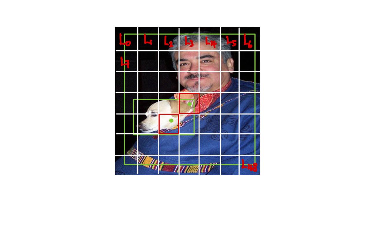
_images/image_1_loss.jpg — Fig. 9 Loss function for a single image.#

Consequently, we define \(\L_i\) to be the loss of each grid cell \(i\) and say that the total loss for a single image is defined as:

(6)#\[\begin{split} \begin{align} \L(\y, \yhat) & \overset{(a)}{=} \sum_{i=1}^{S=7}\sum_{j=1}^{S=7} \L_{ij}(\y_{ij}, \yhat_{ij}) \\ & \overset{(b)}{=} \sum_{i=1}^{S^2=49} \L_i(\y_i, \yhat_i) \\ & \overset{(c)}{=} \sum_{i=0}^{S^2=48} \L_i(\y_i, \yhat_i) \\ \end{align} \end{split}\]

but recall that the equation \((a)\) is not used by us as it is more cumbersome in notations, but just remember that equation \((a)\) and \((b)\) are equivalent. Lastly, because we are dealing with python, we start our indexing from 0, hence the equation \((c)\). Do not get confused!

Equation (6) merely sums up the loss for 1 single image, however, in deep learning, we also have the concept of batch size, where an additional batch size dimension is added. Rest assured it is as simple as summing over the batches and averaging over batch only and will be shown in code later.

(7)#\[\begin{split} \begin{align} \L(\y, \yhat) & \overset{(d)}{=} \dfrac{1}{\text{Batch Size}} \sum_{k=0}^{\text{Batch Size}}\L(\y^{k}, \yhat^{k}) \\ \end{align} \end{split}\]

Loss for a Single Grid Cell in a Single Image#

The simplications in the previous sections allow us to better appreciate what each equation in the loss function mean.

We will also make some very rigid assumptions:

Intuition

Before we look at the seemingly scary formula, let us first think retrospectively on what the loss should penalize/maximize.

The loss should penalize the model if the predicted bounding box x-y coordinates is far away from the ground truth.
The loss should penalize the model if the predicted bounding box width and height is far away from the ground truth.
The loss should penalize the model if the predicted bounding box has low confidence that the grid cell has an object where in fact there is an object. This means the model is not confident enough to predict that this grid cell has an object.
The loss should penalize the model if the predicted bounding box has high confidence that the grid cell has an object where in fact there is no object.
The loss should penalize the model if the predicted bounding box is not predicting the correct class.

The Formula#

In the previous section, equation (6) is the loss function for a single image. We now define \(\L_i(\y_i, \yhat_i)\), the loss of each grid cell \(i\)

(8)#\[\begin{split} \begin{align} \L_i(\y_i, \yhat_i) & \overset{(a)}{=} \color{blue}{\lambda_\textbf{coord} \sum_{j=1}^{B=2} \1_{ij}^{\text{obj}} \lsq \lpar x_i - \hat{x}_i^j \rpar^2 + \lpar y_i - \hat{y}_i^j \rpar^2 \rsq} \\ & \overset{(b)}{+} \color{blue}{\lambda_\textbf{coord} \sum_{j=1}^{B=2} \1_{ij}^{\text{obj}} \lsq \lpar \sqrt{w_i} - \sqrt{\hat{w}_i^j} \rpar^2 + \lpar \sqrt{h_i} - \sqrt{\hat{h}_i^j} \rpar^2 \rsq} \\ & \overset{(c)}{+} \color{green}{\sum_{j=1}^{B=2} \1_{ij}^{\text{obj}} \lpar \conf_i - \confhat_i^j \rpar^2} \\ & \overset{(d)}{+} \color{green}{\lambda_\textbf{noobj}\sum_{j=1}^{B=2} \1_{ij}^{\text{noobj}} \lpar \conf_i - \confhat_i^j \rpar^2} \\ & \overset{(e)}{+} \color{red}{\obji \sum_{c \in \cc} \lpar \p_i(c) - \phat_i(c) \rpar^2} \\ \end{align} \end{split}\]

where

We removed the outer summation \(\sum_{i=1}^{S^2=49}\) as we are only looking at one grid cell \(i\).
\(\mathbb{1}_{i}^{obj}\) is \(1\) when there is a ground truth object in cell \(i\) and \(0\) otherwise.
\(\mathbb{1}_{ij}^{obj}\) denotes that the \(j\)th bounding box predictor in cell \(i\) is matched to ground truth object. This is not easy to understand.
- What this means in our context is that for any grid cell \(i\), there are \(B=2\) bounding box predictors;
- Then, \(\mathbb{1}_{ij}^{obj}\) is \(1\) if it fulfills two conditions:
- Firstly, there is a ground truth object in cell \(i\).
- Secondly, if the first point is true, then out of the \(B=2\) bounding box predictors, only one of them is matched to the ground truth object. We index the 2 bounding box predictors with \(j\), and the one that is matched to the ground truth object will have \(\mathbb{1}_{ij}^{obj}=1\), and the other one will have \(\mathbb{1}_{ij}^{obj}=0\), essentially only taking the matched bounding box predictor into account.
- Remember the matching is done by checking which of the \(B=2\) predicted bounding box has the highest IOU score with the ground truth bounding box.
- This is why the notation has a summation \(\sum_{j=1}^{B=2}\), we are looping over the \(B=2\) bounding box predictors to see which one is matched to the ground truth object.

\[\begin{split} \1_{ij}^{\text{obj}} = \begin{cases} 1 & \textbf{if the ith grid cell has a ground truth obj and jth predictor is matched}\\ 0 & \textbf{otherwise} \end{cases} \end{split}\]

\(\mathbb{1}_{ij}^{noobj}\) is the opposite of \(\mathbb{1}_{ij}^{obj}\), where it is \(1\) when there is no ground truth object in cell \(i\) and the \(j\)th bounding box predictor in cell \(i\) has the highest IOU score among all the predictors of this cell when compared to the ground truth. More on this later as there can be a few interpretations.
Note carefully \(j\) in this context is the indices of the bounding box predictors in each grid cell i.e. in \(\bhat^1\) is the 1st predicted bounding box and the 1 refers to the index \(j=1\).
A constant on what is matched with an object mean? -> it means the bipartite matching algorithm discussed in the previous section.
Last but not least, the \(\xx_i\), \(\yy_i\), \(\ww_i\), \(\hh_i\) are the ground truth bounding box coordinates and \(\hat{\xx}_i^j\), \(\hat{\yy}_i^j\), \(\hat{\ww}_i^j\), \(\hat{\hh}_i^j\) are the predicted bounding box coordinates, both for the grid cell \(i\);
The \(\conf_i\) and \(\confhat_i^j\) are the ground truth confidence score and the predicted confidence score respectively, both for the grid cell \(i\);
The \(\p_i(c)\) and \(\phat_i(c)\) are the ground truth probability of the class \(c\) and the predicted probability of the class \(c\) respectively, both for the grid cell \(i\);

Example with Numbers Part I#

To be honest, I never understood the above equations without the help of numbers. So let us look at some numbers. Let’s zoom in on how to calculate loss for one grid cell \(i\). And for continuity, we will use the \(i=30\) grid cell as an example, the one which the dog is located in.

We will use back the dataframe row which represent the grid cell \(i=30\), for both the ground truth and the predicted bounding boxes.

	x_i^1	y_i^1	w_i^1	h_i^1	conf_i^1	x_i^2	y_i^2	w_i^2	h_i^2	conf_i^2	p_1	p_2	p_3	p_4	p_5	p_6	p_7	p_8	p_9	p_10	p_11	p_12	p_13	p_14	p_15	p_16	p_17	p_18	p_19	p_20
30	0.409	0.277	0.416	0.262	1.0	0.409	0.277	0.416	0.262	1.0	0.0	0.0	0.0	0.0	0.0	0.0	0.0	0.0	0.0	0.0	0.0	1.0	0.0	0.0	0.0	0.0	0.0	0.0	0.0	0.0

	xhat_i^1	yhat_i^1	what_i^1	hhat_i^1	confhat_i^1	xhat_i^2	yhat_i^2	what_i^2	hhat_i^2	confhat_i^2	phat_1	phat_2	phat_3	phat_4	phat_5	phat_6	phat_7	phat_8	phat_9	phat_10	phat_11	phat_12	phat_13	phat_14	phat_15	phat_16	phat_17	phat_18	phat_19	phat_20
30	-0.483	-0.351	-0.595	0.018	0.162	2.688	2.002	-1.169	-4.592	0.758	-0.232	0.527	-0.256	-0.283	0.382	-0.166	-0.071	-0.175	0.147	0.017	-0.415	1.163	-0.043	-0.095	0.132	-0.106	0.269	0.092	-0.085	0.584

In (8), we first see the first equation \((a)\). Let us forget \(\lambda_\textbf{coord}\) for now and just focus on the summand.

Inside the summand, there is the indicator function \(\mathbb{1}_{ij}^{obj}\), and by definition, we first check if there is a ground truth object in the grid cell \(i=30\).
We do know that there is a ground truth object in the grid cell \(i=30\) as the dog is located in this grid cell, as a priori knowledge. But the code does not. It suffices to check the 5th element in the ground truth bounding box coordinates, corresponding to the confidence score \(\conf_{30}\) in the dataframe. By construction in Definition 6, the confidence score is 1 if there is a ground truth object in the grid cell, and 0 otherwise. So a quick look at the dataframe tells us that \(\conf_{30}=1\). So we can proceed.
Next, the matching algorithm happens by means of looping through the \(B=2\) bounding box predictors in the grid cell \(i=30\). However, we soon realize this is not very easily done in code because at each iteration \(j\) over \(B=2\), we are only able to compute the iou(b, bhat) for the \(j\)th bounding box predictor in the grid cell \(i=30\), but unable to deduce if the current iou is the highest. We can of course find a way to store the highest iou, but to make explanation easier, we will remove this loop!

The Formula Modified#

As mentioned in point 3, the observant reader would have realized that the summation \(\sum_{j=1}^{B=2}\) can be refactored out of the equation. This is because for each grid cell \(i\), there is only one unique bounding box predictor that is matched to the ground truth object. The other bounding box predictor(s) in that same grid cell \(i\) will get the cold shoulder since \(\mathbb{1}_{ij}^{obj}=0\), resulting the summand to be \(0\). Further, it is easier to illustrate the loss function with the summation refactored out in code. Let’s again take the liberty to modify slightly the notation to make it more explicit.

Let \(\jmax\) be the index of the bounding box with the IOU score with the ground truth \(\y_i\) in grid cell \(i\). More concretely, \(\jmax\) is our survivor out of the \(B=2\) bounding box predictors in the grid cell \(i\), the one that got successfully matched to the ground truth object in the grid cell \(i\).

Definition 8 (\(\jmax\))

\(\jmax\) is the index in the \(B\) predicted bounding boxes which has the highest IOU score with the ground truth \(\y_i\) in grid cell \(i\).

To be more concise, the IOU score is computed between \(\b_i\) and \(\bhat_i^j\) for \(j=1,2\) as IOU score is a function of the 4 bounding box coordinates.

\[ \jmax = \underset{j \in \{1,2\}}{\operatorname{argmax}} \textbf{IOU}(\b_i, \bhat_i^j) \]

Then we define the new loss function \(\L_i\) for each grid cell \(i\) as follows:

Definition 9 (\(\L_i\) Modified!)

The modified loss function \(\L_i\) for each grid cell \(i\) is defined as follows:

(9)#\[\begin{split} \begin{align} \L_i(\y_i, \yhat_i) & \overset{(a)}{=} \color{blue}{\lambda_\textbf{coord} \cdot \obji \lsq \lpar x_i - \hat{x}_i^{\jmax} \rpar^2 + \lpar y_i - \hat{y}_i^{\jmax} \rpar^2 \rsq} \\ & \overset{(b)}{+} \color{blue}{\lambda_\textbf{coord} \cdot \obji \lsq \lpar \sqrt{w_i} - \sqrt{\hat{w}_i^{\jmax} } \rpar^2 + \lpar \sqrt{h_i} - \sqrt{\hat{h}_i^{\jmax} } \rpar^2 \rsq} \\ & \overset{(c)}{+} \color{green}{\obji \lpar \conf_i - \confhat_i^{\jmax} \rpar^2} \\ & \overset{(d)}{+} \color{green}{\lambda_\textbf{noobj} \cdot \nobji \lpar \conf_i - \confhat_i^{\jmax} \rpar^2} \\ & \overset{(e)}{+} \color{red}{\obji \sum_{c \in \cc} \lpar \p_i(c) - \phat_i(c) \rpar^2} \\ \end{align} \end{split}\]

thereby collapsing the equation to checking only two conditions:

\(\obji\) is \(1\) when there is an object in cell \(i\) and \(0\) elsewhere
\(\1_{i}^{\text{noobj}}\) is \(1\) when there is no object in cell \(i\) and \(0\) elsewhere
\(\y_i\) is exactly as defined in Definition 6’s equation (3).
\(\yhat_i\) is exactly as defined in Definition 7’s equation (4).

The most significant change is that we are going to pre-compute the IOU score between the ground truth \(\y_i\) (\(\b_i\)) with each of the \(B=2\) bounding box predictors \(\bhat_i^j\) (\(j=1,2\)) in the grid cell \(i\), and then pick the bounding box predictor \(\bhat_i^j\) with the highest IOU score and denote the index to be \(\jmax\).

Recap on the Modified Loss Function#

Before we dive into numbers, let’s first recap the loss function for a single grid cell \(i\).

Let’s briefly go through this term by term, bearing in mind that we are talking about 1 single grid cell and not the whole image.

The first part of the equation in (5) computes the loss between the predicted bounding box \(\xx-\yy\) offsets \((\xxhat_i, \yyhat_i)\) and the ground-truth bounding box \(\xx-\yy\) offsets \((\xx_i, \yy_i)\).
- However, we are referring to the original yolo loss function here, which sums up the total loss for a single image. In code however, we want to first compute the loss for each grid cell in a single image, and then sum up the losses for all grid cells in the image.
- Therefore, we will use the our Definition 9, a modified version to find the loss for each grid cell in a single image.
- In the modified version, we see that the first part of the equation (9) computes the loss between the ground truth bounding box \(\xx-\yy\) offsets \((\xx_i, \yy_i)\) and the matched predicted bounding box \(\xx-\yy\) offsets \((\xxhat_i^{\jmax}, \yyhat_i^{\jmax})\).
- Remember carefully that the model predicts two bounding boxes for each grid cell, and we need to match the ground truth bounding box with the predicted bounding box that has the highest IoU with the ground truth bounding box.
- We multiply the loss by a constant \(\lambda_\text{coord}=5\) to ensure that this equation does not get drowned out by the fact that most grid cells do not contain an object. In our example, out of 49 grid cells, only 2 grid cells contains ground truth objects.
- Most importantly, this equation only gets computed for grid cells that contain a ground truth object, as indicated by \(\obji\).
The second part of the equation in (5) computes the loss between the predicted bounding box \(\ww-\hh\) dimensions \((\wwhat_i, \hhhat_i)\) and the ground-truth bounding box \(\ww-\hh\) dimensions \((\ww_i, \hh_i)\).
- Again, we are referring to the original yolo loss function here, which sums up the total loss for a single image. In code however, we want to first compute the loss for each grid cell in a single image, and then sum up the losses for all grid cells in the image.
- Therefore, we will use the our Definition 9, a modified version to find the loss for each grid cell in a single image.
- In the modified version, we see that the second part of the equation (9) computes the loss between the ground truth bounding box \(\ww-\hh\) dimensions \((\ww_i, \hh_i)\) and the matched predicted bounding box \(\ww-\hh\) dimensions \((\wwhat_i^{\jmax}, \hhhat_i^{\jmax})\).
- There is a catch, however. We are actually computing the loss between the square root of the ground truth bounding box \(\ww-\hh\) dimensions \(\sqrt{\ww_i}, \sqrt{\hh_i}\) and the square root of the matched predicted bounding box \(\ww-\hh\) dimensions \(\sqrt{\wwhat_i^{\jmax}}, \sqrt{\hhhat_i^{\jmax}}\). The reason can be found in my Intuition: Parametrization of Bounding Box.
- Remember carefully that the model predicts two bounding boxes for each grid cell, and we need to match the ground truth bounding box with the predicted bounding box that has the highest IoU with the ground truth bounding box.
- We multiply the loss by a constant \(\lambda_\text{coord}=5\) to ensure that this equation does not get drowned out by the fact that most grid cells do not contain an object. In our example, out of 49 grid cells, only 2 grid cells contains ground truth objects.
- Most importantly, this equation only gets computed for grid cells that contain a ground truth object, as indicated by \(\obji\).
The third part of the equation in (5) computes the loss between the predicted object confidence \(\confhat_i\) and the ground-truth object confidence \(\conf_i\).
- We see that the third part of the equation (9) computes the loss between the ground truth object confidence \(\conf_i\) and the matched predicted object confidence \(\confhat_i^{\jmax}\).
- Remember carefully that the model predicts two object confidences for each grid cell, and we need to match the ground truth object confidence with the predicted object confidence that has the highest IoU with the ground truth bounding box.
- Recall that the ground truth \(\conf_i\) is defined as 1 if the grid cell contains an object, and 0 otherwise initially, but during loss computation, \(\conf_i\) is defined to be the IoU between the ground truth bounding box and the predicted bounding box that has the highest IoU, as seen in Definition 5. But for our code, we will just use conf_i = 1 or conf_i = 0 for simplicity.
- Most importantly, this equation only gets computed for grid cells that contain a ground truth object, as indicated by \(\obji\).
The fourth part of the equation in (5) computes the loss between the predicted object confidence \(\confhat_i\) and the ground-truth object confidence \(\conf_i\) when the grid cell does not contain an object.
- Even though in our fourth part of the equation (9), we put a \(\jmax\) subscript, but in code we actually compute the loss for all predicted bounding boxes in the grid cell. This is logical as well because if the grid cell does not contain an object, then the predicted bounding boxes should both have a low object confidence and be penalized to tell the model that the grid cell does not contain an object.
- We multiply the loss by a constant \(\lambda_\text{noobj}=0.5\) to ensure that this equation does not get drowned out by the fact that most grid cells do not contain an object. We do not want this term to overpower the gradients for the cells containing objects as this could lead to model instability and be harder to optimize [Redmon et al., 2016].
The fifth part of the equation in (5) computes the loss between the predicted class probabilities \(\phat_i\) and the ground-truth class probabilities \(\p_i\).
- We see that the fifth part of the equation (9) computes the loss between the ground truth class probabilities \(\p_i\) and the matched predicted class probabilities \(\phat_i\).
- Note that \(\p_i\) and \(\phat_i\) are both vectors of length \(C\), where \(C\) is the number of classes. They are not scalars unlike the previous equations.
- Note that we do not have \(\jmax\) here because both predicted bounding boxes share the same class probabilities.
- Most importantly, this equation only gets computed for grid cells that contain a ground truth object, as indicated by \(\obji\). This is why the author call them conditional probabilities, \(\mathcal{P} \left( \p_i \mid \obji = 1 \right)\). It is only computed conditionally on the fact that the grid cell contains an object.

In summary:

After the forward pass, the model will have encoded the ground truth \(\b_30\) and the two predicted bounding boxes \(\bhat_i^1\) and \(\bhat_i^2\). Our first step is to determine which of the two predicted bounding boxes is the best match for the ground truth, the filtering process is done by the IOU metric.

Assuming that the matching is done, for the predicted boxes that are matched to ground truth boxes the loss function is minimizing the error between those boxes, maximising the objectness confidence, and maximising the liklihood of the correct class (which is shared between two boxes). For all predicted boxes that are not matched with a ground truth box, it is minimising the objectness confidence, but ignoring the box coordinates and class probabilities [Turner, 2021].

Examples with Numbers Part II#

"""
Implementation of Yolo Loss Function from the original yolo paper
"""
import torch
from torch import nn
# from utils import intersection_over_union, bmatrix
import numpy as np
import pandas as pd

# reshape to [49, 30] from [7, 7, 30]
class YOLOv1Loss2D(nn.Module):
    def __init__(
        self,
        S: int,
        B: int,
        C: int,
        lambda_coord: float = 5,
        lambda_noobj: float = 0.5,
    ) -> None:
        super().__init__()
        self.S = S
        self.B = B
        self.C = C
        self.lambda_coord = lambda_coord
        self.lambda_noobj = lambda_noobj
        # mse = (y_pred - y_true)^2
        # FIXME: still unclean cause by right reduction is not sum since we are
        # adding scalars, but class_loss uses vector sum reduction so need to use for all?
        self.mse = nn.MSELoss(reduction="none")
        
        self.device = torch.device("cuda" if torch.cuda.is_available() else "cpu")

    def _initiate_loss(self) -> None:
        """Initializes all the loss values to 0.
        
        Note:
            This is an important step if not the current batch loss will be added to the
            next batch loss which causes error in `loss.backward()`.
        """
        # bbox loss
        self.bbox_xy_offset_loss = 0
        self.bbox_wh_loss = 0

        # objectness loss
        self.object_conf_loss = 0
        self.no_object_conf_loss = 0

        # class loss
        self.class_loss = 0

    def compute_xy_offset_loss(
        self,
        x_i: torch.Tensor,
        xhat_i: torch.Tensor,
        y_i: torch.Tensor,
        yhat_i: torch.Tensor,
    ) -> torch.Tensor:
        """Computes the loss for the x and y offset of the bounding box."""
        x_offset_loss = self.mse(x_i, xhat_i)
        y_offset_loss = self.mse(y_i, yhat_i)
        xy_offset_loss = x_offset_loss + y_offset_loss
        return xy_offset_loss

    def compute_wh_loss(
        self,
        w_i: torch.Tensor,
        what_i: torch.Tensor,
        h_i: torch.Tensor,
        hhat_i: torch.Tensor,
        epsilon: float = 1e-6,
    ) -> torch.Tensor:
        """Computes the loss for the width and height of the bounding box.
        
        Note:
            The width and height are predicted as the square root of the width and height
            and absolute values are applied to the predictions as they are unbounded
            below and can be numerically unstable.
        """
        w_loss = self.mse(torch.sqrt(w_i), torch.sqrt(torch.abs(what_i + epsilon)))
        h_loss = self.mse(torch.sqrt(h_i), torch.sqrt(torch.abs(hhat_i + epsilon)))
        wh_loss = w_loss + h_loss
        return wh_loss

    def compute_object_conf_loss(
        self, conf_i: torch.Tensor, confhat_i: torch.Tensor
    ) -> torch.Tensor:
        """Computes the loss for the object confidence when there is really an object."""
        return self.mse(conf_i, confhat_i)

    def compute_no_object_conf_loss(
        self, conf_i: torch.Tensor, confhat_i: torch.Tensor
    ) -> torch.Tensor:
        """Computes the loss for the object confidence when there is no object."""
        return self.mse(conf_i, confhat_i)

    def compute_class_loss(self, p_i: torch.Tensor, phat_i: torch.Tensor) -> torch.Tensor:
        """Computes the loss for the class prediction.

        Note:
            Instead of looping C number of classes, we can use self.mse(p_i, phat_i)
            as the vectorized version.
        """
        total_class_loss = 0
        for c in range(self.C):
            total_class_loss += self.mse(p_i[c], phat_i[c])
        return total_class_loss

    # fmt: off
    def forward(self, y_trues: torch.Tensor, y_preds: torch.Tensor) -> torch.Tensor:
        """Forward pass of the loss function.

        Args:
            y_trues (torch.Tensor): The ground truth tensor of shape (bs, S, S, 5B + C).
            y_preds (torch.Tensor): The predicted tensor of shape (bs, S, S, 5B + C).

        Returns:
            total_loss_averaged_over_batch (torch.Tensor): The total loss averaged over the batch.
        """
        self._initiate_loss()                                                                       # reset loss values
        
        y_trues = y_trues.reshape(-1, self.S * self.S, self.C + self.B * 5)                         # (4, 49, 30)
        y_preds = y_preds.reshape(-1, self.S * self.S, self.C + self.B * 5)                         # (4, 49, 30)

        batch_size = y_preds.shape[0]                                                               # 4

        for batch_index in range(batch_size):                                                       # for each image in batch 
            y_true = y_trues[batch_index]                                                           # y:    (49, 30)
            y_pred = y_preds[batch_index]                                                           # yhat: (49, 30)

            for i in range(self.S * self.S):                                                        # i is the grid cell index [0, 48] 
                y_true_i = y_true[i]                                                                # y_i:    (30,) or (1, 30)
                y_pred_i = y_pred[i]                                                                # yhat_i: (30,) or (1, 30)
                
                indicator_obj_i = y_true_i[4] == 1                                                  # this is $\obji$ and checking y_true[i, 4] is sufficient since y_true[i, 9] is repeated

                if indicator_obj_i:                                                                 # here equation (a), (b), (c) and (e) of the loss equation on a single grid cell.
                    b = y_true_i[0:4]                                                               # b:    (4,) or (1, 4)
                    bhat_1 = y_pred_i[0:4]                                                          # bhat1: (4,) or (1, 4)
                    bhat_2 = y_pred_i[5:9]                                                          # bhat2: (4,) or (1, 4)
                    
                    x_i, y_i, w_i, h_i = b                                                          # x_i, y_i, w_i, h_i: (1,)
                    # at this stage jmax is not known yet.
                    xhat_i1, yhat_i1, what_i1, hhat_i1 = bhat_1                                     # xhat_i1, yhat_i1, what_i1, hhat_i1: (1,)
                    xhat_i2, yhat_i2, what_i2, hhat_i2 = bhat_2                                     # xhat_i2, yhat_i2, what_i2, hhat_i2: (1,)
                    
                    conf_i, confhat_i1, confhat_i2 = y_true_i[4], y_pred_i[4], y_pred_i[9]          # conf_i, confhat_i1, confhat_i2: (1,)
                    
                    p_i, phat_i = y_true_i[10:], y_pred_i[10:]                                      # p_i, phat_i: (20,) or (1, 20)

                    # area of overlap
                    iou_b1 = intersection_over_union(b, bhat_1, bbox_format="yolo")                 # iou of b and bhat1
                    iou_b2 = intersection_over_union(b, bhat_2, bbox_format="yolo")                 # iou of b and bhat2

                    if iou_b1 > iou_b2:
                        # conf_i = max_{bhat \in {bhat_1, bhat_2}} IoU(b, bhat)
                        # however I set conf_i = y_true_i[4] = 1 here as it gives better results for our case
                        xhat_i_jmax, yhat_i_jmax, what_i_jmax, hhat_i_jmax, confhat_i_jmax = xhat_i1, yhat_i1, what_i1, hhat_i1, confhat_i1
                        confhat_i_complement = confhat_i2
                    else:
                        xhat_i_jmax, yhat_i_jmax, what_i_jmax, hhat_i_jmax, confhat_i_jmax = xhat_i2, yhat_i2, what_i2, hhat_i2, confhat_i2
                        confhat_i_complement = confhat_i1
                        
                    
                    self.bbox_xy_offset_loss += self.lambda_coord * self.compute_xy_offset_loss(x_i, xhat_i_jmax, y_i, yhat_i_jmax)                 # equation 1
                    self.bbox_wh_loss += self.lambda_coord * self.compute_wh_loss(w_i, what_i_jmax, h_i, hhat_i_jmax)                               # equation 2
                    self.object_conf_loss += self.compute_object_conf_loss(conf_i, confhat_i_jmax)                                                  # equation 3

                    # mention 2 other ways
                    # iou比较小的bbox不负责预测物体，因此confidence loss算在noobj中，注意，对于标签的置信度应该是iou2
                    # we can set conf_i = iou_b2 as well as the smaller of the two should be optimized to say there exist no object instead of proposing something.
                    # we can set conf_i = 0 as well and it will work.
                    # TODO: comment for blog if uncomment it performs a bit better early.
                    # self.no_object_conf_loss += self.lambda_noobj * self.compute_no_object_conf_loss(conf_i=torch.tensor(0., device="cuda"), confhat_i=confhat_i_complement)
                    self.class_loss += self.compute_class_loss(p_i, phat_i)                                                                               # equation 5
                else:
                    for j in range(self.B):
                        self.no_object_conf_loss += self.lambda_noobj * self.compute_no_object_conf_loss(conf_i=y_true_i[4], confhat_i=y_pred_i[4 + j * 5]) # equation 4

        total_loss = (
            self.bbox_xy_offset_loss
            + self.bbox_wh_loss
            + self.object_conf_loss
            + self.no_object_conf_loss
            + self.class_loss
        )

        # if dataloader has a batch size of 2, then our total loss is the average of the two losses.
        # i.e. total_loss = (loss1 + loss2) / 2 where loss1 is the loss for the first image in the
        # batch and loss2 is the loss for the second image in the batch.
        total_loss_averaged_over_batch = total_loss / batch_size
        # print(f"total_loss_averaged_over_batch {total_loss_averaged_over_batch}")

        return total_loss_averaged_over_batch

	x_i^1	y_i^1	w_i^1	h_i^1	conf_i^1	x_i^2	y_i^2	w_i^2	h_i^2	conf_i^2	p_1	p_2	p_3	p_4	p_5	p_6	p_7	p_8	p_9	p_10	p_11	p_12	p_13	p_14	p_15	p_16	p_17	p_18	p_19	p_20
30	0.409	0.277	0.416	0.262	1.0	0.409	0.277	0.416	0.262	1.0	0.0	0.0	0.0	0.0	0.0	0.0	0.0	0.0	0.0	0.0	0.0	1.0	0.0	0.0	0.0	0.0	0.0	0.0	0.0	0.0

	xhat_i^1	yhat_i^1	what_i^1	hhat_i^1	confhat_i^1	xhat_i^2	yhat_i^2	what_i^2	hhat_i^2	confhat_i^2	phat_1	phat_2	phat_3	phat_4	phat_5	phat_6	phat_7	phat_8	phat_9	phat_10	phat_11	phat_12	phat_13	phat_14	phat_15	phat_16	phat_17	phat_18	phat_19	phat_20
30	-0.483	-0.351	-0.595	0.018	0.162	2.688	2.002	-1.169	-4.592	0.758	-0.232	0.527	-0.256	-0.283	0.382	-0.166	-0.071	-0.175	0.147	0.017	-0.415	1.163	-0.043	-0.095	0.132	-0.106	0.269	0.092	-0.085	0.584

1st image in the batch has objects in row 24 and 30 (human, dog at 3,3 and 2,4)

line x-x:
- y_trues consists of \(4\) ground truth bounding boxes of shape (4, 49, 30).
- y_preds consists of \(4\) predicted bounding boxes of shape (4, 49, 30).
- These two variables are zipped into batches of \(N\) for deep learning computation but we will only focus on the first image of the batch.
line x:
- batch_size is the number of images in the batch, in this case \(N = 4\).
line x says for batch_index in range(batch_size): will loop over the first image in the batch.
- when batch_index=0:
  - y_true is the ground truth matrix of shape (49, 30);
  - y_pred is the predicted matrix of shape (49, 30);
  - loop over grid cells from 0 to 48:
    - when i=0:
      - y_true_i is the ground truth matrix of shape (1, 30) for the cell i=0;
      - y_true_i = [0, 0, 0, ..., 0] a zero vector because there is no ground truth object in the cell i=0 by Definition 6.
      - y_pred_i is the predicted matrix of shape (1, 30) for the cell i=0;
        
        [ 0.9248, -0.1671, 0.1906, 0.7233, 0.2136, 1.0013, 0.1228, 0.0577, 0.5615, -0.1186, -0.5857, -0.0233, -0.1024, -0.1603, -0.4082, 0.5643, -0.1626, 0.2941, -0.2064, -0.6844, -0.2154, 0.3397, 0.4247, 0.1387, -0.4165, -0.2329, 0.2822, 0.5175, 0.3936, 0.0671]
      - indicator_obj_i corresponds to \(\obji\) in the equation above and is equal to \(0\) when there is no object in cell \(i=0\). In this grid cell i=0, this will be equal to 0.
      - line x says if indicator_obj_i == 1: will be False because there is no object in cell i=0.
      We do not explicitly define indicator_noobj_i to correspond to \(\nobji\) but it is equal to \(1\) since there is no object in cell \(i=0\). This means that it will not go through the if clause in line ?? and will go through else clause in line ?? and will compute the loss for the no object equation at \(d\) equation above.
      - So we will skip over all lines in the if clause and go to else clause.
      - No object loss: line xx-xx means we are looping over the 2 bounding boxes in cell \(i=0\).
        
        Loop over \(j=0\)
        
        y_true[i, 4] is the confidence score of the 1st bounding box in cell \(i=0\).
        
        It is equal to \(0\) since there is no object in cell \(i=0\) by Definition 5.
        
        y_pred[i, 4] is the confidence score of the 1st bounding box in cell \(i=0\).
        
        We see that the model predicted 0.2136 for the first bounding box j=0.
        
        We will compute the mean squared error between the ground truth confidence score and the predicted confidence score of the 1st predicted bounding box.
        
        \(0.5 \times (0.2136 - 0)^2 = 0.5 \times 0.04562496 = 0.02281248\)
        
        Loop over \(j=1\)
        
        We still use y_true[i, 4] because the y_true[i, 9] is same as y_true[i, 4] by construction in Definition 6.
        
        y_pred[i, 9] is the confidence score of the 2nd bounding box in cell \(i=0\).
        
        We see that the model predicted -0.1186 for the second bounding box j=1.
        
        We will compute the mean squared error between the ground truth confidence score and the predicted confidence score of the 2nd predicted bounding box.
        
        \(0.5 \times (-0.1186 - 0)^2 = 0.5 \times 0.01406596 = 0.00703298\)
      - Finally we have \(0.02281248 + 0.00703298 = 0.02984546\) for the no object loss in cell \(i=0\).
      - At this point the total loss for grid cell i=0 is done:
        
        self.bbox_xy_offset_loss = 0
        
        self.bbox_wh_loss = 0
        
        self.object_conf_loss=0
        
        self.no_object_conf_loss=0.02984546
        
        self.class_loss=0
    - when i=30:
      - y_true_i = [0.4093, 0.2770, 0.4164, 0.2620, 1, 0.4093, 0.2770, 0.4164, 0.2620, 1, 0, 0, 0, 0, 0, 0, 0, 0, 0, 0, 0, 1, 0, 0, 0, 0, 0, 0, 0, 0]
      - y_pred_i = [-0.4827, -0.3511, -0.5949, 0.0183, 0.1622, 2.6878, 2.0020, -1.1686, -4.5915, 0.7578, -0.2317, 0.5274, -0.2556, -0.2830, 0.3817, -0.1655, -0.0712, -0.1746, 0.1467, 0.0166, -0.4146, 1.1629, -0.0429, -0.0952, 0.1323, -0.1055, 0.2692, 0.0923, -0.0845, 0.5842]
      - indicator_obj_i corresponds to \(\obji\) in the equation above and is equal to \(1\) since there is an object in cell \(i=30\).
      - So equations a, b, c and e goes into the if clause and equation d goes into the else clause.
      - Some variables below:
      b_gt: [0.4093485 0.27699995 0.4164306 0.262 ] b_pred_1: [-0.48271456 -0.3510531 -0.5948943 0.01832254] b_pred_2: [ 2.6877854 2.0019963 -1.1685951 -4.591512 ] x_i, y_i, w_i, h_i = 0.4093485, 0.27699995, 0.4164306, 0.262 xhat_i1, yhat_i1, what_i1, hhat_i1 = -0.48271456, -0.3510531, -0.5948943, 0.01832254 xhat_i2, yhat_i2, what_i2, hhat_i2 = 2.6877854, 2.0019963, -1.1685951, -4.591512 conf_1, confhat_i1, confhat_i2 = 1, 0.1622, 0.7578
      - Then in line x-x, we compute iou_b1 and iou_b2 which are the intersection over union between the ground truth bounding box and the predicted bounding boxes. This is for the Bipartite matching part when we choose which predictor \(\jmax\) to use to compute the loss with the ground truth.
      - In line x-x, we do a simple inequality check (note this is not scalable if you have more than 2 bounding box predictors per grid cell) to see which bounding box predictor has the highest intersection over union with the ground truth bounding box. In this case it is the 2nd bounding box predictor j=1 since iou_b2 > iou_b1.
      So:
      xhat_i_jmax, yhat_i_jmax, what_i_jmax, hhat_i_jmax = xhat_i2, yhat_i2, what_i2, hhat_i2
      - self.bbox_xy_offset_loss:
        
        x_offset_loss -> \((0.4093484878540039 - 2.6877853870391846)^2 = 5.19127470357\)
        
        y_offset_loss -> \((0.27699995040893555 - 2.0019962787628174)^2 = 2.97561233283\)
        
        self.bbox_xy_offset_loss -> \(5 \times (5.19127470357 + 2.97561233283) = 5 \times 8.1668870364 = 40.8344\)
      - self.bbox_wh_loss:
        
        w_loss -> \((\sqrt{0.41643059253692627} - \sqrt{\abs{-1.1685951}})^2 = 0.1898357414137847\)
        
        h_loss -> \((\sqrt{0.262} - \sqrt{\abs{-4.591512}})^2 = 2.659906617074438\)
        
        self.bbox_wh_loss -> \(5 \times (0.1898357414137847 + 2.659906617074438) = 14.2487\)
      - self.object_conf_loss:
        
        self.object_conf_loss -> \((1 - 0.7578)^2 = 0.05864378437399864\)
      - self.no_object_conf_loss:
        
        self.no_object_conf_loss -> \(0\)
        
        Note that in my code we have self.no_object_conf_loss += self.lambda_noobj * self.compute_no_object_conf_loss(conf_i=torch.tensor(0., device="cuda"), confhat_i=confhat_i_complement) which also computes the no object loss for the other bounding box predictor in the cell. But we won’t calculate it here. The reason some people do that is they want to penalize the network for predicting something for the other bounding box predictor even though there is an object in that grid cell. In other words, they want it to specialize for predictor \(\jmax\).
      - self.class_loss:
        
        This part is simple, we just compute the mean squared error between the ground truth class and the predicted class for each element.

References#

Sphinx#

$ pip uninstall sphinx-proof
$ pip install -U git+https://github.com/executablebooks/sphinx-proof.git@master

For the newest assumptions directives.

Citations#

1(1,2,3,4,5): Joseph Redmon, Santosh Divvala, Ross Girshick, and Ali Farhadi. You only look once: unified, real-time object detection. 2016 IEEE Conference on Computer Vision and Pattern Recognition (CVPR), 2016. doi:10.1109/cvpr.2016.91.
2(1,2,3): Harry Turner. Yolo v1. 2021. URL: https://www.harrysprojects.com/articles/yolov1.html.

1: https://www.harrysprojects.com/articles/yolov1.html

YOLOv1 Explained

YOLOv1

Contents

YOLOv1#

Unified Detection#

Model Architecture#

Python Implementation#

Model Summary#

Backbone#

Head#

Anchors and Prior Boxes#

Bounding Box Parametrization#

YOLOv1 Encoding Setup#

Notations and Definitions#

Sample Image#

Bounding Box Parametrization#

Loss Function#

Other Important Notations#

From 3D Tensor to 2D Matrix#

Construction of Ground Truth Matrix#

Construction of Prediction Matrix#

Loss Function#

Bipartite Matching#

Total Loss for a Single Image#

Loss for a Single Grid Cell in a Single Image#

The Formula#

Example with Numbers Part I#

The Formula Modified#

Recap on the Modified Loss Function#

Examples with Numbers Part II#

References#

Sphinx#

Citations#